MATHEMATICS
Restriction implies decoupling, but in a different dimension
Changkeun Oh’s 2025 theorem connects Fourier restriction in one dimension of ambient space to decoupling in another, with a precise conditional step.
Research checked
Newest cited publication
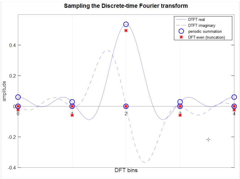
Discrete samples of a Fourier transform provide a basic visual introduction to frequency analysis; the restriction and decoupling estimates here concern substantially richer settings.
Bob K / Wikimedia Commons. Unchanged original image. · Image source · CC0 1.0

Two major tools in harmonic analysis study how waves add together, but they package the question differently. Fourier restriction asks how oscillations associated with a curved frequency surface spread through physical space. Decoupling asks whether the combined wave can be bounded by contributions from smaller frequency patches. A short paper posted by Changkeun Oh on March 18, 2025, establishes a precise bridge: restriction for a paraboloid in d-dimensional ambient space implies a particular decoupling theorem in ambient dimension 2d minus one. The dimension change is central to the result, and so is the word implies.
A surface of frequencies, many possible waves
A Fourier extension operator starts with a function assigning amplitudes to points on a frequency surface. It combines the corresponding oscillations into a function of physical position. For a paraboloid, one can describe the surface by taking several coordinates and appending a signed sum of their squares. Choosing all signs alike gives the usual curved bowl; mixed signs give a hyperbolic paraboloid. Curvature affects how the resulting oscillations reinforce or cancel.
To see why a norm matters, imagine two oscillations with equal amplitude. At one location their phases agree and the amplitude doubles. Elsewhere they may cancel. A bound for a global p norm measures the distribution of these effects, with larger p placing more emphasis on unusually large amplitudes. An estimate is therefore more informative than saying that cancellation happens somewhere. It controls the cumulative cost of concentration across space.
The theorem changes the ambient dimension
Oh proves that the restriction conjecture for the relevant paraboloid in ambient dimension d yields the stated l-p decoupling estimate in ambient dimension 2d minus one. The paper also gives an unconditional consequence in ambient dimension three, using the already established restriction result in ambient dimension two. It is an alternative route to an existing decoupling theorem, rather than a proof that restriction is solved in all dimensions.
Substituting values prevents a common misreading. Taking d equal to two sends the conclusion to dimension three. Taking d equal to three sends it to dimension five. The second substitution is a conditional implication when its restriction hypothesis has not been supplied. A logical arrow does not manufacture its starting premise. This simple bookkeeping is especially important when several papers discuss the same conjecture using surface dimension in one place and ambient dimension in another.
Why l-two and l-p are different claims
Decoupling separates a function into pieces whose Fourier supports occupy small patches. One then compares the p norm of their sum with a sequence norm of the p norms of the pieces. Bourgain and Demeter's earlier l-two decoupling theorem is foundational here, but the sequence norm in the 2025 bridge is l-p. These labels describe different quantities and should not be exchanged because both results involve a paraboloid.
For N pieces all having norm one, the l-two total is the square root of N, while the l-four total is the fourth root of N. With sixteen pieces these are four and two, respectively. A theorem using the smaller sequence total may include a compensating power of the scale parameter. Comparing only the sequence norm while ignoring that scale factor gives a false impression of relative strength. A fair comparison fixes the frequency geometry, patch size, exponent range and allowed growth of the constant.
A square root appears for a geometric reason
The natural patch width near a paraboloid is tied to its quadratic shape. If a tangential coordinate changes by h, the departure from its tangent plane is of order h squared. To keep that departure within a normal thickness of one over R, take h of order one over the square root of R. For R equal to ten thousand, the normal scale is one ten-thousandth and the corresponding tangential scale is one hundredth.
This calculation is independent of the difficult inequality: it explains the scale at which the inequality is posed. It also explains why rescaling can be productive. A small curved patch, after translating and adjusting its tangent plane, resembles the original paraboloid at another resolution. Quadratic surfaces preserve this relationship especially cleanly. The technical challenge is to use this geometric repetition while keeping track of constants as the pieces are divided repeatedly.
Related routes do not collapse into one theorem
Wang and Wu's separate research program uses decoupling together with two-ends Furstenberg inequalities to obtain restriction estimates. Their paper formulates a conjectural geometric input and proves a planar version that yields a three-dimensional restriction improvement. This provides a useful contrast to Oh's arrow from restriction to decoupling: the hypotheses, geometry and dimensions differ, so the pair does not establish an unrestricted equivalence between the entire theories.
Demeter's earlier work on decoupling beyond the canonical setup similarly distinguishes large ensemble decoupling from tight decoupling and connects them to different restriction phenomena. The lesson is methodological. When a field has several estimates with similar names, a new connection should be recorded as a specific map between statements. Listing its domain and conclusion is more reliable than announcing that two broad areas have become the same subject.
Why an alternative proof earns attention
Suppose a difficult estimate is known through a long argument using several deep ingredients. A second derivation that begins from a better understood theorem can reveal which parts of the conclusion follow from a common mechanism. It may improve teaching, suggest extensions or expose a hidden constraint. None of those benefits requires the numerical exponent itself to improve. This is the appropriate way to appreciate the three-dimensional consequence of Oh's note.
A careful reader can audit the bridge in four passes. First identify the signed quadratic surface. Next check whether d denotes ambient dimension. Then distinguish the physical-space p norm from the sequence norm over patches. Finally record the scale loss, including any arbitrarily small positive exponent. These checks are elementary to state but difficult proofs depend on all of them. Once that bookkeeping is secure, the larger research question becomes clearer: which forms of lower-dimensional wave control can be transferred through slicing and rescaling into higher-dimensional control? The 2025 result gives one exact answer, with its premises still attached.
The arithmetic behind the dimension lift
The dimension formula can be checked against the critical exponents. In the notation of Oh's statement, the restriction boundary in ambient dimension d is 2 + 2/(d − 1). The upper endpoint of the relevant decoupling range in ambient dimension D is 2 + 4/(D − 1). Substituting D = 2d − 1 gives D − 1 = 2d − 2 = 2(d − 1), so the two numerical expressions agree. This arithmetic does not prove the implication, but it explains why that particular dimension relationship is plausible.
For d equal to two, both boundary expressions give four after the conclusion is placed in dimension three. For d equal to three, both give three after the conclusion is placed in dimension five. One must still distinguish an open restriction range from how an endpoint is handled in a decoupling statement, including the permitted small scale loss. Matching one number is a consistency test, not permission to erase those details. It also provides an efficient error check when reading summaries: a purported dimension transfer that changes these exponent relationships needs a different argument and cannot simply be identified with the theorem discussed here.
Sources & further reading
Primary papers, project documentation, and research releases used in this article. Publication dates below refer to the sources themselves.
- On decoupling and restriction estimatesarXivPublished Checked
- The proof of the l² Decoupling ConjecturearXivPublished Checked
- Restriction estimates using decoupling theorems and two-ends Furstenberg inequalitiesarXivPublished Checked
- Beyond canonical decouplingarXivPublished Checked
FOLLOW THE QUESTION
Explore mathematics