MATHEMATICS
Random Growth on a Ring Gets a General Starting Shape
A 2026 probability preprint constructs periodic KPZ fixed-point distributions from general starting profiles, extending beyond specially solvable initial shapes.
Research checked
Newest cited publication
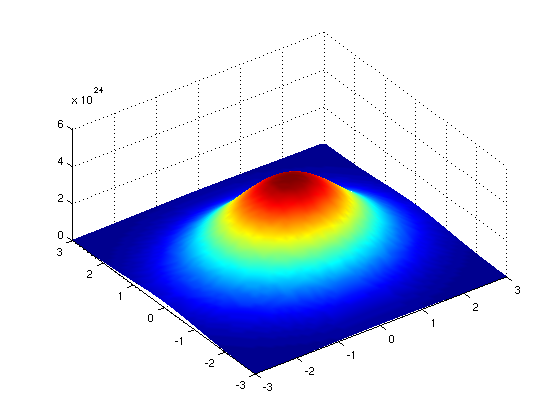
A smooth Gaussian surface introduces a basic random-distribution model; the periodic growth profiles and KPZ limits discussed here have their own probability laws.
Michael Hardy / Wikimedia Commons. Unchanged original image. · Image source · Public domain (released by the creator)

A traffic jam on a circular road eventually feels the size of the road. Before that happens, a short stretch may resemble an infinite highway; afterward, a disturbance can return to the region where it began. Random growth models have an analogous crossover, and it changes which scaling limit is appropriate. In a preprint first submitted on 2 March 2026 and substantially revised on 21 July, Jinho Baik, Yuchen Liao and Zhipeng Liu construct a periodic Kardar–Parisi–Zhang fixed point for general admissible initial profiles through consistent space-time distributions. The result extends the range of starting shapes beyond earlier special cases. Its mathematical interest lies as much in the meaning of a random evolving field as in the formulas used to describe it.
A ring of particles is a growth model
The underlying system is periodic totally asymmetric simple exclusion, often abbreviated PTASEP. Sites lie on a ring, with at most one particle at each site. A particle tries to jump in one direction, and an occupied target blocks the jump. Those local restrictions create collective effects even when the attempted moves are driven by simple independent clocks. A height representation translates the particle arrangement and cumulative current into an evolving interface. The ring geometry means that the same finite set of vacancies and particles repeatedly constrains the dynamics.
For an original small example, place three particles on six sites, initially occupying sites zero, one and three. If motion is clockwise, the particle at zero is blocked by the one at one. The particle at one can move into two, and the particle at three can move into four. After either move, the list of available moves changes. Writing an equation that treats the three particles as independent random walkers would therefore produce the wrong process. The interaction is encoded by the forbidden occupancy, rather than by an explicit attractive force.
Which limit sees the circumference?
A scaling limit requires deciding what grows and what is observed. Increasing the number of sites while watching only a fixed microscopic time does not reveal the same phenomenon as increasing time together with the circumference. In the Kardar–Parisi–Zhang picture, fluctuations in height, spatial correlation length and elapsed time are associated with characteristic exponents one third, two thirds and one. These exponents describe a coordinated magnification, not three separate claims that every random process has those powers.
Here is a scaling argument rather than a proof. Suppose correlations spread over a length proportional to time to the power two thirds. A ring of circumference L begins to matter when that length reaches L. Solving time to the power two thirds equals L gives time of order L to the power three halves. Height fluctuations of order time to the power one third then have size L to the power one half. This is why studying a ring near its relaxation scale differs from simply wrapping an infinite-line picture around a circle after the calculation.
This heuristic also specifies a useful size comparison. Doubling circumference would multiply the corresponding relaxation time by 2 to the power three halves, about 2.83, and the fluctuation height scale by the square root of two, about 1.41. Holding time proportional only to circumference would therefore compare different positions within the crossover. These ratios follow from the assumed exponents; they are not new measured constants. A simulation intended to visualize a fixed scaling regime should preserve those relationships before interpreting changes in a histogram as a change of limiting law.
General initial data still has a definition
The 2026 preprint treats microscopic configurations approximating a periodic upper semicontinuous profile, in the specified hypograph topology. The particle density, N_L divided by L, stays bounded away from both zero and one as circumference L increases. The profile may take minus infinity, but cannot be identically minus infinity. The authors obtain limiting multipoint laws and prove their consistency, defining a periodic random field. Their new representations encode initial data through random-walk hitting times, including a first hit constrained to occur at or after a full period. These are preprint results for the stated approximation regime, not a proof that every growth model shares this periodic limit.
Upper semicontinuity has a useful geometric interpretation. At a point, the profile cannot sit strictly below the limiting values approaching from nearby points. A downward puncture in an otherwise flat graph violates that condition, whereas an isolated upward peak can satisfy it. The hypograph consists of points lying on or below the graph. Describing convergence through these regions preserves the barrier geometry that matters to a path trying to hit the profile. This explanation clarifies the language of the assumption without replacing its precise definition.
Why a collection of formulas is not enough
Imagine claiming to describe three binary random variables A, B and C. Suppose each pair is said to disagree with probability one. The three pairwise descriptions cannot all arise from a single triple: if A differs from B and B differs from C, then A equals C. This elementary contradiction shows why formulas for separate groups of observations do not automatically define a coherent random object. Their overlapping predictions must agree.
For a random height field, one may request the joint distribution at two positions and one time, or at several positions across several times. Removing one requested observation should recover the formula for the remaining observations. Reordering observations should merely relabel coordinates. Repeated observations should agree with themselves. These compatibility requirements are what consistency means in this setting. A limit for each separately chosen event is already useful, but a consistent family provides the pieces of one field. Establishing continuous sample paths or a specific path-space convergence statement would require additional assertions; those should never be silently inserted into a finite-dimensional result.
A profile is information, not decoration
Start one ring in an alternating particle-vacancy arrangement and another with most particles packed together. Both can have the same particle density. Nevertheless, one begins with many immediately available jumps, while the other begins with a broad blocked region and a moving boundary. A single density value does not specify this information. General initial profiles let a theorem ask which aspects survive after the appropriate rescaling, rather than requiring the experiment to begin with a specially chosen flat or stepped arrangement.
The earlier paper Periodic TASEP with general initial conditions, first posted on 20 December 2019, supplied finite-time space-time formulas for arbitrary periodic initial configurations. Its relaxation-scale analysis imposed further conditions verified for selected profiles. The distinction between an exact finite-size formula and an asymptotic theorem is essential: a formula can be valid while taking its limit remains difficult. On the infinite line, Matetski, Quastel and Remenik’s The KPZ fixed point, first posted on 30 December 2016, established the corresponding central random evolution using exact transition descriptions. The periodic geometry asks another limiting question.
A barrier gives a useful way to think
For an explanatory construction, let a random path move above a chosen graph and record the first moment it reaches the region below it. Raising part of the graph can make an earlier hit possible; moving a peak can alter which part of the path is sampled. This converts a whole starting shape into a stopping rule. On a periodic graph, distinguishing an unrestricted hit from a hit at or after one period retains information about winding around the geometry. This is an interpretation of why such representations are useful, rather than a derivation of the paper’s kernels.
The practical next step for a reader is to compare several admissible profiles under one fixed normalization. Keep particle density, circumference scaling and observation times explicit, then ask which joint probabilities change when the starting profile changes. Simulations can help display that dependence, but small rings cannot certify the limiting field. The advance is a broader mathematical starting point: the periodic theory can now address an entire class of profiles through compatible distributions. Questions about further universality, stronger process convergence or applications to real traffic need their own hypotheses and evidence.
Sources & further reading
Primary papers, project documentation, and research releases used in this article. Publication dates below refer to the sources themselves.
- Periodic KPZ fixed point with general initial conditionsarXivPublished Checked
- Periodic TASEP with general initial conditionsarXivPublished Checked
- The KPZ fixed pointarXivPublished Checked
FOLLOW THE QUESTION
Explore mathematics