MATHEMATICS
Noise Can Fix a Distribution Without Fixing a Path
A 2026 stochastic-analysis preprint constructs rough drifts with unique weak laws but pathwise nonuniqueness, locating a sharp boundary for regularization by noise.
Research checked
Newest cited publication
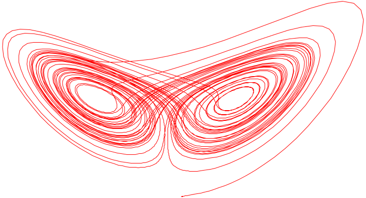
A trajectory from a deterministic nonlinear system provides visual context for paths through state space; the article examines a separate stochastic uniqueness question.
Cepheus / Wikimedia Commons. Unchanged original image. · Image source · Public domain (released by the creator)

Adding randomness to an ill-behaved differential equation can make its solutions more orderly. This phenomenon, called regularization by noise, is one of stochastic analysis’s most striking reversals of ordinary intuition. But there are several meanings of a unique solution. An equation can determine one probability law while still allowing different trajectories under the same driving noise. A preprint submitted by Elias Hess-Childs and Keefer Rowan on 26 April 2026 constructs exactly this separation for a carefully specified rough drift in two dimensions. The result puts a sharp obstruction beside classical positive uniqueness theorems. Understanding the obstruction requires distinguishing the randomness used to construct a coefficient, the noise driving the equation and the information available to a solution.
What does it mean to know the solution?
Write an additive stochastic equation in integral form: X(t) equals its initial position plus the time integral of u(s, X(s)) plus W(t) minus W(0). The function u is the drift, and W is the driving noise. A weak solution constructs a compatible probability model for the required objects. Weak uniqueness concerns the probability law. A strong solution is built measurably from the prescribed noise and initial data, with the appropriate nonanticipation requirement. The adjective strong describes that information structure, rather than numerical accuracy or greater physical force.
Pathwise uniqueness asks whether two compatible solutions starting together and driven by the same noise on the same probability space must coincide. Path-by-path uniqueness is another statement: fix almost every driving path and ask whether the resulting deterministic integral equation has only one allowed trajectory. The quantifiers and information restrictions differ. A. M. Davie’s 2007 paper proved a strong positive path-by-path result for additive Brownian noise with bounded Borel drift. That statement supplies an important baseline, not a guarantee for every rougher class.
A waiting-time example explains the difficulty
Consider the deterministic equation x prime equals twice the square root of the larger of x and zero, starting from zero. For any waiting time a greater than or equal to zero, keep x equal to zero until a, then set x(t) equal to (t minus a) squared. Before departure both sides vanish. After departure the derivative is twice (t minus a), matching the right-hand side. Every waiting time therefore gives a solution. This elementary example is not the vector field constructed in the 2026 paper.
Now suppose two solutions of an additive-noise equation share W. Subtracting their integral equations cancels the explicit W term, leaving the integral of the difference between the drifts evaluated at their different positions. Cancellation does not make the solutions equal: the drift still depends on where each path goes. If the drift were Lipschitz in position with a suitable integrable bound, an integral inequality would force the difference to remain zero. Rough coefficients remove precisely the control used in that familiar argument. Noise can restore uniqueness in some settings, but the conclusion needs a theorem.
What the April preprint actually constructs
Theorem 1.3 of Hess-Childs and Rowan’s preprint constructs a two-dimensional divergence-free velocity field for every rho strictly between zero and one half. It has a uniform negative-regularity C to the power minus rho bound and belongs to time-integrable continuous spatial fields. For independent Brownian driving noise, it has a unique weak solution but pathwise nonuniqueness on every initial time interval. Randomness is used in constructing the field; an appropriate deterministic realization can then be fixed.
These conditions matter. The theorem is not about a generic smooth velocity, and the stated two-dimensional construction is not a one-dimensional example. The noise is independent of the constructed field. Negative spatial regularity does not here mean abandoning every pointwise interpretation: the additional integrability and continuity condition permits the integral equation formulation used by the authors. The article is a preprint, so the correct claim is that its authors present a proof of this sharpness result, rather than that every conceivable uniqueness question has been settled.
Why a coefficient norm can hide large oscillations
An original oscillatory example clarifies negative regularity. Take a sine wave whose frequency increases through positive integers k. A negative Hölder-type norm discounts high spatial frequencies. Heuristically, a wave with amplitude a and frequency k contributes at scale a times k to a negative power. Choosing amplitude k raised to the power rho/2 makes the pointwise amplitude grow, while its C to the power minus rho contribution decreases like k raised to the power -rho/2. This is a scaling illustration, not an exact norm identity or the research construction.
The example explains why a uniform negative-regularity bound cannot be substituted for a uniform amplitude bound. Oscillations can cancel when tested on a coarse spatial scale even though local velocities are large. Time dependence can add another layer: a field can be integrable in time without being uniformly bounded near the initial time. A claim that Brownian motion regularizes bounded measurable drifts therefore does not automatically cover every coefficient that is small in a negative spatial norm. The spaces encode genuinely different information about the coefficient.
For a numerical version of the frequency illustration, choose rho = 1/4 and frequency k = 256. The chosen amplitude k to the power rho divided by two is 256 to the power one eighth, which equals two. The frequency-discounted contribution is then two times 256 to the power minus one quarter, which equals one half. Increasing frequency has doubled the visible amplitude while halving this scale-weighted quantity relative to frequency one. Constants in an actual function-space norm depend on its definition, so these figures are an illustration of powers rather than a quoted sharp bound. They make the issue concrete: a discretization that reports a small coarse norm can still encounter large velocities at spatial scales that its grid barely resolves.
Identical statistics do not identify a trajectory
For a simple probability analogy, take one fair coin U. Let A equal U, and consider two constructions of a second fair coin B. In the first, B equals U; in the second, B equals one minus U. The individual distributions of A and B are identical in both constructions, but their coupling changes completely. This is not a stochastic differential equation counterexample. It is a warning that knowing marginal distributions does not specify how two random objects are related on one shared probability space.
In an equation driven by specified noise, the coupling with that noise is part of the question. A conditional distribution of the solution given the driving path can retain nontrivial randomness even when an overall law is uniquely determined. A strong solution, by contrast, is a measurable choice from the available driving information. One must not infer the absence of all strong solutions merely from any isolated failure of pathwise uniqueness. The new construction has more structure than that inference: its theorem separates the relevant solution notions within the precise additive-noise setting.
The gap between weak and pathwise theories
Butkovsky and Mytnik’s Weak uniqueness for singular stochastic equations, first posted on 22 May 2024 and revised on 31 March 2025, provides another perspective. For an additive fractional Brownian equation with Hurst parameter H between zero and one half and suitable distributional drift of regularity alpha, it establishes weak uniqueness when alpha exceeds one half minus 1/(2H). The work combines generalized coupling ideas with stochastic sewing. It is a different theorem, with different coefficient and noise assumptions, rather than a direct restatement of the Brownian counterexample.
As a numerical reading aid, choose H = 1/4. The stated weak threshold becomes alpha greater than minus 3/2. Substituting that value is straightforward arithmetic, but concluding pathwise uniqueness would require an additional result. This distinction matters for approximation: convergence of simulated histograms can support a conjectured law while concealing differences between trajectories sharing one noise sample. The next informative question is therefore not simply whether noise helps. It is which noise, which coefficient space, which solution concept and which kind of convergence have actually been controlled.
Sources & further reading
Primary papers, project documentation, and research releases used in this article. Publication dates below refer to the sources themselves.
- Sharp pathwise nonuniqueness for additive SDEsarXivPublished Checked
- Weak uniqueness for singular stochastic equationsarXivPublished Checked
- Uniqueness of solutions of stochastic differential equationsarXivPublished Checked
FOLLOW THE QUESTION
Explore mathematics