MATHEMATICS
Computing a matrix square root without spending double precision everywhere
A July 2026 preprint combines a cheaper Schur decomposition with careful correction. Its central challenge is that matrices do not multiply like scalars.
Research checked
Newest cited publication
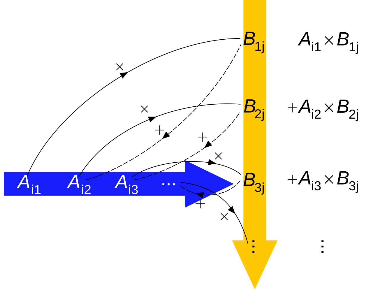
A matrix illustration introduces the structured numerical objects manipulated when computing matrix square roots with different arithmetic precisions.
Maschen / Wikimedia Commons. Wikimedia-generated PNG rendering of the SVG; no editorial changes. · Image source · Public domain (released by the creator)

A square root sounds like a single button on a calculator. For a matrix, it becomes a problem involving an entire system of interacting entries. Taking the square root of each entry does not generally produce a matrix whose square equals the original. Researchers must choose a meaningful root, compute it reliably, and check the answer without spending more time than the problem deserves. A preprint posted on July 14, 2026, by Bowen Gao, Daniel Kressner, and Meiyue Shao explores an appealing division of labor: do expensive preparation in lower precision, then use more accurate arithmetic to identify and repair the remaining error. Its interest lies in the structure of that repair.
A root is another transformation
Consider the diagonal matrix with entries four and nine. Its principal square root has diagonal entries two and three. Applying that root twice stretches the first coordinate by four and the second by nine. This familiar case can hide the difficulty. For the upper triangular matrix with diagonal entries four and nine and upper right entry five, the root instead has diagonal entries two and three and upper right entry one. Squaring it produces an upper right entry of two times one plus one times three, which is five. The entries cooperate through multiplication.
That example also explains why a branch must be selected. Changing signs on diagonal roots can produce different solutions, and some combinations make intermediate equations difficult or impossible. The principal root is the branch whose eigenvalues lie in the open right half of the complex plane when the input has no eigenvalues on the nonpositive real axis. The official SciPy documentation describes its square root routine through the Schur method. This is established numerical machinery, rather than an invention of the 2026 paper.
What the cheaper preparation buys
A Schur decomposition changes coordinates until a matrix becomes triangular, using an orthogonal or unitary change of basis. Triangular matrices retain the information needed for the square root while allowing entries or blocks to be solved in a controlled order. The earlier work of Edvin Deadman, Nicholas Higham, and Rui Ralha explains how blocking rearranges this task around efficient matrix multiplication. The distinction matters: two algorithms can perform similar numbers of arithmetic operations and still run at very different speeds because they reuse cached data differently.
The July preprint computes this preparation in reduced precision and reuses its factors during correction. Its reported timing advantage is an experimental result on the tested architectures, rather than a promise for every machine. A practical comparison must include coordinate transformations, conversion costs, and the eventual accuracy test. If the initial preparation is already cheap, or if accurate corrections require many extra rounds, the apparent bargain can disappear. Lower precision is a resource allocation decision, not an accuracy setting that can simply be turned down globally.
Deriving the correction by multiplication
An independent calculation shows what a correction must accomplish. Let X be an approximate root and let E be a small correction. Multiplication gives (X + E)² = X² + XE + EX + E². If the residual is R = A − X², canceling the first order error asks for XE + EX = R. This is a Sylvester equation: the unknown matrix appears on both sides of known matrix factors. The quadratic remainder E² becomes small as the approximation improves. This derivation requires no assumption that X and E commute.
For a concrete example, start with X having diagonal entries two and three and an unwanted upper right entry 0.01, while A is diagonal with entries four and nine. The upper right residual is −0.05. A correction with upper right entry −0.01 solves the relevant equation because two times −0.01 plus three times −0.01 equals −0.05. In this special triangular example, the correction squares to zero, so the repair is exact in exact arithmetic. It demonstrates the role of both multiplication orders without pretending to reproduce a performance experiment.
The residual needs a clearer view
Suppose a measuring device reports distances only to the nearest centimeter. Repeatedly asking that same device whether a position is wrong by a millimeter cannot improve the answer. Residual arithmetic has a related limitation. Once X² is close to A, forming A − X² involves subtracting nearly equal quantities. Low precision can erase the very discrepancy that the correction is supposed to address. Computing the check in higher precision preserves information that a less accurate inner solve can still use productively.
The analogy has limits: floating point errors depend on the sizes and operations involved, not on one fixed measuring interval. Nevertheless, it explains why an algorithm can tolerate inexpensive corrections while demanding a careful residual and update. It also explains why stopping merely because successive answers look identical is weak evidence. Rounded updates may stop changing before the desired residual is achieved. A reliable implementation needs an accuracy target tied to the original matrix, a maximum iteration count, and a way to report failure to reach the target.
A small residual is only part of accuracy
Take the positive scalar a = 0.0001. Its positive root is 0.01. If the squared value is perturbed by a tiny amount δa, the first order change of the root is approximately δa divided by 0.02. Now compare a = 100, whose root changes by approximately δa divided by twenty. The same absolute perturbation has a very different absolute effect. Relative error introduces another normalization, so absolute and relative conditioning must not be mixed in the same claim.
For matrices, the Sylvester operator E ↦ XE + EX describes this sensitivity. A residual can be tiny while the corresponding forward error remains significant if that operator nearly loses invertibility. Symmetric positive definite inputs offer more structure because their eigenvectors can be chosen orthonormally and their root eigenvalues are positive. General matrices introduce additional sensitivity. The new paper separates these cases in its analysis. Readers should therefore resist extending a favorable conclusion for the positive definite case to every nonsymmetric matrix.
What an honest comparison should record
Imagine testing two square root routines on a family of matrices. Recording only runtime rewards an algorithm that stops too early. Recording only the residual can conceal differences in conditioning. A useful report should include the matrix sizes, structure, chosen arithmetic formats, relative residual, reference based forward error when available, number of correction steps, and total elapsed time. It should disclose whether decomposition costs are included and whether either routine benefits from cached work or different thread counts.
The choice of test matrices matters as much as the timing apparatus. Diagonal examples help validate arithmetic but tell little about nonnormal behavior. Random dense examples cover only the distributions that generated them. Matrices approaching a branch boundary probe an entirely different difficulty. These are methodological recommendations from the mathematics of the problem, rather than additional results claimed by the preprint. A convincing future implementation would make such cases reproducible and expose its stopping decisions instead of reporting a single favorable speed ratio.
A precise route to spending precision
The development is a preprint as of the October 18, 2026 research cutoff. Its contribution should be read as a carefully analyzed algorithm with numerical evidence, rather than a universal replacement for established library routines. In particular, the cost of solving correction equations must be balanced against the savings from preparing reusable factors. Accuracy conditions and the behavior of difficult general matrices remain central to judging where the method is suitable.
The broader lesson is useful beyond this one function. Precision belongs to operations and information flows. Some steps construct a coarse but valuable model; others diagnose the remaining error; still others apply a repair whose own inaccuracies can be corrected later. Matrix square roots make that principle unusually visible because the correction equation exposes exactly what scalar intuition misses. Spending fewer accurate operations can be mathematically justified, provided the algorithm preserves a more accurate way to ask whether it has actually finished.
Sources & further reading
Primary papers, project documentation, and research releases used in this article. Publication dates below refer to the sources themselves.
- A mixed precision algorithm for the matrix square rootarXivPublished Checked
- Blocked Schur Algorithms for Computing the Matrix Square RootUniversity of Manchester MIMS EPrintsChecked
- sqrtm — SciPy v1.18.0 ManualSciPyChecked
FOLLOW THE QUESTION
Explore mathematics