MATHEMATICS
Moving fewer bytes without losing a linear solve
An October 2026 preprint studies lower precision storage in matrix splitting iterations, connecting memory traffic, convergence, and accurate residual corrections.
Research checked
Newest cited publication
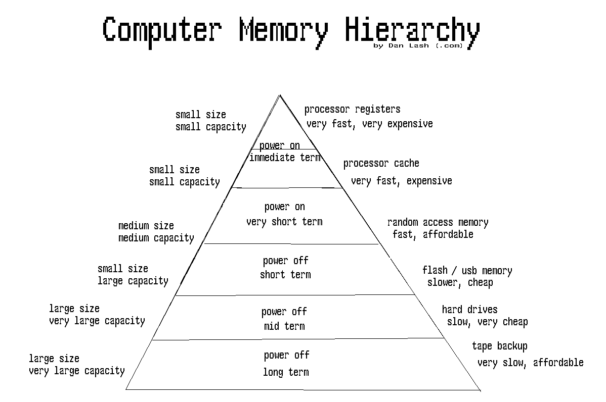
A computer-storage hierarchy illustrates why data movement matters alongside arithmetic when mixed-precision matrix splitting is used in a linear solve.
Danlash · Image source · Public domain

A fast processor can spend much of a numerical calculation waiting for data. When a sparse matrix is repeatedly applied to a vector, the machine may move far more information than it processes arithmetically. Reducing the stored precision can help, but a linear solver must still solve the intended equations. A preprint submitted on October 5, 2026, by Neil Lindquist, David Appelhans, Charles W. Jackson, and Joseph M. Derlaga examines this tradeoff for matrix splitting methods. The immediate subject is familiar iterative algebra. The more general question is how to reduce memory traffic without allowing the numerical shortcut to change the answer beyond the requested accuracy.
A splitting turns one problem into repeated easier ones
Write A = M + N, where systems involving M are comparatively easy to solve. Then Ax = b can be approached through the iteration x next = M⁻¹(b − Nx). The formula says to treat the N part using the current guess and solve the remaining M part more directly. For Jacobi iteration, M is the diagonal. For Gauss–Seidel, M includes a triangular portion. An implementation usually solves with M rather than explicitly constructing its inverse.
Take A with rows (4, 1) and (1, 3), and b = (1, 2). Jacobi iteration updates the first coordinate to (1 − y)/4 and the second to (2 − x)/3 using the previous coordinates. Starting at zero gives (1/4, 2/3), then (1/12, 7/12). The exact solution is (1/11, 7/11), as direct substitution verifies. This is an illustrative calculation, not a test case attributed to the new paper. It shows how a sequence of cheap updates can approach a coupled answer.
The update must actually reduce error
Subtract the exact solution from the update equation. The error is multiplied by −M⁻¹N at every exact arithmetic step. Convergence therefore depends on this iteration matrix rather than on the mere existence of a splitting. For the two coordinate example, one error component becomes minus one quarter of the other, and the other becomes minus one third of the first. After two updates, each original component has been multiplied by one twelfth. That is a concrete contraction.
A different matrix can behave very differently. If the off diagonal couplings overwhelm the diagonal, the same recipe can amplify errors. Lower precision cannot rescue an inherently divergent exact iteration merely by making it cheaper. Conversely, an iteration that barely contracts has little room for new perturbations. This is why a performance argument needs a convergence argument alongside it. Counting fewer bytes explains a possible speed benefit; it does not establish that the required number of iterations remains similar.
Precision can be a storage decision
Imagine storing one hundred million matrix values. Eight byte values occupy eight hundred million bytes; two byte values occupy two hundred million. If every iteration reads those values, the potential traffic difference is substantial. A sparse format also stores row and column information, so reducing value size by a factor of four does not reduce the complete matrix representation by the same factor. Temporary arrays, vector reads, and cache behavior contribute further costs. These simple counts explain the opportunity without predicting a machine benchmark.
The October preprint studies selective reduced precision storage within matrix splittings, including off diagonal blocks. Across the full tested sample, the geometric mean speedups for half precision are 1.27 for Jacobi and 1.08 for Gauss–Seidel. The larger figures of 1.60 and 1.25 exclude cases that slowed down; some configurations therefore lose performance. The paper also reports an overall speedup of 1.14 for the tested OVERFLOW application. These measurements depend on the tested matrices and configuration. Improving an inner iteration and improving an entire application remain distinct achievements.
Rounding the matrix can change the fixed point
Suppose an off diagonal entry of one is stored as 1 + ε. An iteration using that stored value may converge perfectly to the solution of a slightly different matrix. More iterations cannot remove an error that is built into the equation being iterated. For the example above, the changed first equation would be 4x + (1 + ε)y = 1. Substituting the original exact solution leaves a discrepancy of ε times 7/11. The altered coefficient causes a nonzero original residual even after the modified iteration settles.
This distinction separates convergence from correctness. A sequence can stabilize and still fail the accuracy target for the original problem. It also explains why a useful implementation retains sufficient information to evaluate the original residual. If only the rounded matrix survives, an accurate residual for the original matrix may no longer be available. The storage policy must therefore be designed together with the correction strategy, rather than bolting a convergence check onto an already irreversible loss of input information.
Refine against the original equation
For an approximate answer x, form r = b − Ax accurately. Seek a correction d satisfying Ad = r, then replace x by x + d. The correction need not be computed perfectly to help. If its remaining error is a fixed fraction of the previous error, repetition can recover additional accuracy. The point is that each new correction is driven by a residual for the original system. This is the basic logic of iterative refinement, whose use of inexpensive inner calculations predates current low precision hardware.
The earlier work of Julie Langou and colleagues explicitly investigated obtaining high precision answers with lower precision arithmetic at selected stages. Eda Oktay and Erin Carson later developed multistage refinement that monitors progress and can switch to a more robust approach. These sources supply context for the 2026 development. They do not imply that one precision combination succeeds for every matrix. Residual quality, correction quality, conditioning, representable range, and stopping decisions all affect the attainable result.
Two separate limits: sensitivity and representable range
A diagonal matrix with entries one and one hundred millionth is invertible, but its two scales are far apart. A small absolute perturbation to the smaller entry can have a large relative effect on its inverse. An inner solve involving such a matrix needs more care than one involving equal diagonal entries. This illustrates why the conditioning of M matters in a splitting method, alongside the contraction of the full iteration. A storage format must preserve the information needed by the easy solve itself.
Range is a separate issue. A format can represent small relative increments around one yet fail to represent a required large magnitude, or can represent a wide range while retaining comparatively few significant bits. Scaling can help keep numbers within range, but it does not by itself guarantee good conditioning or remove the need for accuracy analysis. Multiplying an entire system by a common nonzero scalar leaves its normwise matrix condition number unchanged, while row or column equilibration can change it. Treating every sixteen bit format as interchangeable therefore misses an important numerical distinction. The correct format depends on the distribution of matrix values and the operations performed on them.
Measure the solve from input to verified answer
Suppose half of an application time is spent in an operation that becomes twice as fast, while the rest is unchanged. The new total time is three quarters of the original, giving a speedup of four thirds. The application cannot become twice as fast under those assumptions. Conversion, residual evaluation, or extra iterations can reduce the gain further. This independent arithmetic explains why an impressive kernel result is insufficient to predict the value of a full solver change.
As of October 18, 2026, the October result is a preprint with theoretical analysis and numerical experiments. A reproducible comparison should record total wall time to the same verified residual, the storage formats, matrix characteristics, conversion overhead, iteration counts, and any failure or fallback. The appealing direction is precise: store selected information more cheaply while preserving an accurate feedback loop. When the assumptions hold, mathematical error analysis makes the memory saving useful. When they fail, a solver should expose that fact rather than quietly returning a cheaper answer to a different equation.
Sources & further reading
Primary papers, project documentation, and research releases used in this article. Publication dates below refer to the sources themselves.
- A Mixed-Precision Model for Matrix-Splitting MethodsarXivPublished Checked
- Multistage Mixed Precision Iterative RefinementarXivPublished Checked
- Exploiting the Performance of 32 bit Floating Point Arithmetic in Obtaining 64 bit Accuracy (Revisiting Iterative Refinement for Linear Systems)University of Tennessee authors; PARA 2006 archiveChecked
FOLLOW THE QUESTION
Explore mathematics