ENGINEERING
GPS Turns Atomic Time into Position Through a Managed Error Budget
GPS connects atomic clocks, orbital predictions and radio measurements. Its landmark achievement is making timing useful while accounting for many different errors.
Research checked
Newest cited publication
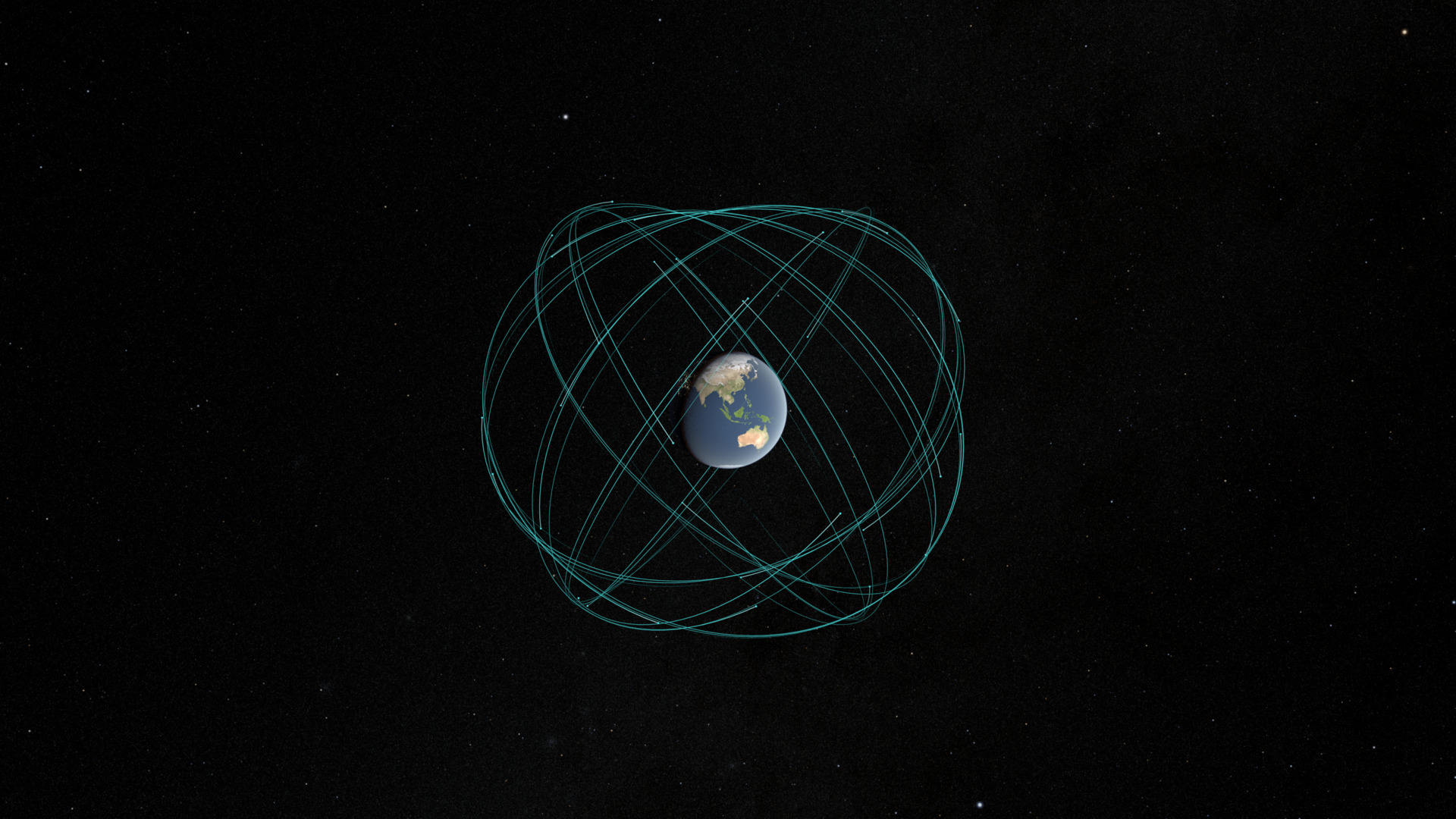
A 2026 NASA visualization illustrates GPS satellite orbits and constellation geometry. It provides a modern explanation of the navigation architecture whose timing and ranging principles are examined in the article.
NASA Scientific Visualization Studio / Kel Elkins (Science and Technology Corporation) · Image source · Public domain (NASA SVS)
A GPS receiver does not discover its location by asking a satellite where the receiver is. It listens to carefully timed broadcasts and solves a measurement problem. That distinction explains both the system’s extraordinary usefulness and its familiar failures near buildings. The landmarks are distributed across a chain: stable clocks, known signal structures, predicted satellite positions, coordinated time, propagation models and receiver calculations. Relativity belongs in that chain, but it does not explain every navigation error. This historical engineering account uses the original NIST receiver analysis, the August 2022 interface specification and official performance documentation to examine how many imperfect measurements become a useful position.
The measured distance contains a clock error
The NIST technical note by Neil Ashby and Marc Weiss describes the basic observation as a pseudorange: a reception-time reading minus a transmitted-time reading, multiplied by the speed of light. It is an apparent range because the receiver’s local clock is not perfectly synchronized with GPS time. Satellite clock offsets and propagation effects also require treatment. A navigation solution normally estimates three spatial coordinates and the receiver’s clock offset using measurements from at least four satellites.
For scale, one nanosecond corresponds to approximately 0.30 metres of light travel. A receiver clock that is one hundred microseconds ahead can therefore add approximately thirty kilometres to every otherwise ideal apparent range. That does not mean the user must be thirty kilometres from the correct position. A shared receiver-clock bias is a separate unknown in the calculation. Confusing it with a different geometric error on every satellite would throw away the structure that makes the system solvable.
Atomic stability must become a reproducible radio measurement
The GPS performance standard describes an onboard atomic frequency standard feeding synthesized clock signals, ranging-code generation and radio transmission. Ground monitoring and uploaded navigation data are also part of the system. An atomic reference supplies a stable basis for timing; it does not independently tell the receiver the satellite’s exact current position or eliminate the need to estimate clock behavior.
The interface specification defines signals that receivers can recognize. A receiver compares the incoming ranging code with a locally generated version and adjusts their alignment. In engineering terms, the receiver turns agreement between patterns into a timing observation. The navigation message provides the additional information needed to interpret that observation. Detecting a carrier, identifying a satellite, tracking a code and calculating a position are related operations, rather than one interchangeable capability.
An illustrative recording helps distinguish them. A precisely sampled radio waveform can contain genuine GPS signals without yielding a useful position immediately: the processing must determine which signals are present, recover their timing relationships and obtain applicable navigation information. A better oscillator helps preserve measurements, but software still has to attach the correct meaning to them.
The fourth unknown is an economical design choice
In an idealized model, each apparent range equals the geometric satellite-to-receiver distance plus a common receiver-clock term. Four independent measurements supply four equations for three coordinates and that clock term. Actual solvers use corrections, additional observations and estimation methods; counting equations alone does not establish a unique, well-conditioned solution.
A simple one-dimensional analogy makes the benefit visible. Put two ideal transmitters at opposite ends of a straight baseline and a receiver between them. With a common clock bias added to both apparent ranges, subtracting the observations cancels that bias and reveals the receiver’s displacement from the midpoint. Adding the observations instead helps identify the common bias when the baseline length is known. This simplified example is not a GPS receiver algorithm, but it shows why sharing an error across measurements can make it estimable.
Geometry still matters. Observations from nearly the same direction supply similar information, so small measurement changes can cause large coordinate changes. More observations help most when they add useful independent directions and reliable measurements, rather than simply increasing a satellite counter on a screen.
The famous thirty-eight microseconds is only the beginning
NIST’s clock explanation gives the familiar approximate daily effects: satellite motion slows clocks by seven microseconds relative to earthbound clocks, while the gravitational difference speeds them by forty-five microseconds. Their net effect is about thirty-eight microseconds per day. These are rounded explanatory values. The interface specification gives a nominal frequency offset of minus 4.4647 parts in ten billion to compensate for the mean relativistic rate difference.
The same specification separately requires a periodic relativistic correction associated with orbital eccentricity. A constant rate adjustment cannot remove a variation that changes around the orbit. Clock bias and drift parameters in the navigation message address still other aspects of satellite timing. Treating all these corrections as one daily subtraction would mix distinct mechanisms and responsibilities.
Multiplying thirty-eight microseconds by light speed gives about 11.4 kilometres of equivalent range. That calculation is useful for appreciating the scale of an untreated timing effect. It is not a prediction that every uncorrected receiver would drift exactly 11.4 kilometres in position each day. A shared timing error can enter the estimated clock offset; differential errors and geometry determine how errors project into the spatial solution.
Transmission and reception happen at different events
Ashby and Weiss emphasize calculating propagation consistently between the satellite’s transmission event and the receiver’s reception event. Earth-fixed coordinates rotate, so taking an ordinary straight-line distance between coordinates expressed at different times in that rotating frame can miss the necessary rotation correction. An equivalent calculation can use a suitable common Earth-centered inertial frame and then transform the result.
For a sense of scale, suppose a signal spends seventy milliseconds in flight. A point moving eastward at an illustrative four hundred metres per second travels twenty-eight metres during that interval. The exact GPS correction depends on satellite and receiver geometry; twenty-eight metres is not a universal correction to apply. The example simply explains why a short radio transit time is still long enough for reference-frame bookkeeping to matter at navigation accuracy.
A coordinate system is therefore part of the measurement definition, not decoration added to a final map. Correct numerical arithmetic cannot rescue a calculation that silently combines positions belonging to incompatible times or frames.
A superb clock cannot remove a reflected radio path
GPS.gov distinguishes broadcast signal accuracy from the user’s resulting accuracy. It identifies atmospheric effects, satellite geometry, blocked signals, reflected paths and receiver design among the relevant factors. This is why an accurate satellite clock and a correct relativistic model do not guarantee an accurate position beside a tall building. Some errors occur after transmission, along the particular route to a particular antenna.
For a deliberately simple reflection example, suppose a signal follows a path thirty metres longer than the unobstructed route. The excess delay is approximately one hundred nanoseconds. A receiver might mistake some of that delay for additional range, depending on the reflected and direct components and its tracking design. The calculation establishes a scale, not a universal multipath error. If the direct path is blocked entirely, averaging more measurements of the wrong path does not automatically recover the missing geometry.
Mitigation must match the mechanism. Frequency diversity can help separate ionospheric delay because that delay depends on radio frequency. It does not make a building transparent. Better antenna placement can improve the available paths without changing an atomic clock. Navigation quality emerges from these different interventions working together.
A performance claim needs its measurement boundary
The April 2020 Standard Positioning Service performance standard separates signal-in-space measures from position and time performance under stated assumptions. Accuracy, availability, continuity and integrity describe different properties. A signal can be available while a particular receiver has poor geometry; a precise estimate can still be unsuitable if a fault is not detected promptly. The standard’s scope and exclusions matter as much as an appealing numerical threshold.
For a device test, this suggests reporting sky visibility, receiver type, frequencies, correction services, antenna location and the reference used to judge error. A ninety-five-percent bound should retain its time interval and population. A result from a stationary, surveyed antenna cannot silently become a promise for a moving phone indoors. The measurement boundary determines what the evidence actually demonstrates.
GPS became a landmark by making a physical model and an operational interface work together at global scale. Atomic clocks are essential, but usefulness arrives through managed uncertainty: knowing which timing effect is already compensated, which observation needs correction, and which local limitation remains. That discipline is what turns radio time into dependable coordinates.
Sources & further reading
Primary papers, project documentation, and research releases used in this article. Publication dates below refer to the sources themselves.
- Global Positioning System Receivers and RelativityNational Institute of Standards and TechnologyPublished Checked
- GPS Interface Specification IS-GPS-200, Revision NUnited States Space ForcePublished Checked
- Global Positioning System Standard Positioning Service Performance Standard, 5th EditionUnited States Department of DefensePublished Checked
- Putting Einstein to the TestNational Institute of Standards and TechnologyPublished Checked
- GPS AccuracyGPS.govChecked
FOLLOW THE QUESTION
Explore engineering