MATHEMATICS
Four Colors, Infinitely Many Maps, and a Finite Proof
The four-color theorem joins a global counting constraint to finite reducibility checks, followed by a formal proof that verifies the computational bridge.
Research checked
Newest cited publication
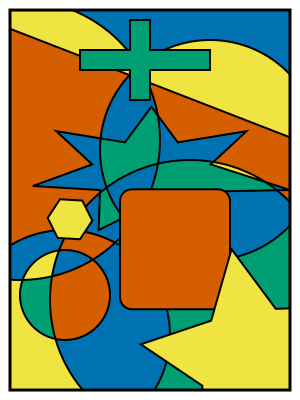
A modern four-color map illustrates the coloring condition: regions sharing a boundary segment receive different colors. Point contacts alone do not create adjacency, and the picture is an example rather than the theorem’s proof.
Inductiveload; original map by Chas zzz brown / Wikimedia Commons. Unchanged original SVG. · Image source · CC BY-SA 3.0

A map may have ten regions or ten million, yet four colors suffice when adjacent regions must differ under the usual planar-map rules. The four-color theorem makes a universal promise, not a prediction that most ordinary maps will be easy to color. Kenneth Appel and Wolfgang Haken announced their computer-assisted proof in 1976; the detailed discharging and reducibility papers appeared in 1977, with John Koch a coauthor of the latter. A separate proof by Neil Robertson, Daniel Sanders, Paul Seymour and Robin Thomas was published in 1997. Georges Gonthier’s later formal proof added another milestone: the mathematics and the computational checks were verified together in Coq. The key is how infinitely many possible maps can be controlled through finite local reasoning.
Specify which objects receive colors
In the finite graph formulation, every loopless planar graph has a proper vertex coloring using at most four colors. Proper means that the endpoints of every edge have different colors. Planar means that the graph can be drawn in the plane without edge crossings, except where edges meet at their endpoints. A self-loop would demand that a vertex differ from itself, explaining why looplessness is part of the statement. Parallel edges impose the same inequality repeatedly and do not introduce that obstruction.
For ordinary region maps, sharing a boundary segment creates adjacency, while touching only at a corner does not. Translating regions into vertices and shared boundaries into edges connects the map picture to graph coloring. A country made of disconnected pieces can change the problem if all pieces are required to share one color. The theorem does not automatically cover that extra constraint. Definitions that seem cosmetic in a picture determine whether the claimed guarantee applies.
Why the number four is sharp
The complete graph on four vertices, K4, is planar: draw a triangle, put the fourth vertex inside, and connect it to all three corners. Every pair of its vertices is adjacent. Three colors cannot suffice, because two of the four vertices would share a color and violate an edge constraint. Four distinct colors work. Thus the theorem cannot be strengthened by replacing four with three, even for very small planar graphs.
The next complete graph, K5, illustrates why planarity matters. It has five vertices and ten edges. A simple planar graph with at least three vertices has at most three times its number of vertices minus six edges, which would allow at most nine here. Hence K5 is nonplanar and is outside the theorem’s hypothesis. Crossing lines in a drawing do not make a graph nonplanar by themselves; what matters is whether some crossing-free drawing exists.
A hypothetical failure has a smallest representative
Suppose a finite planar graph requiring more than four colors existed. Choose a counterexample minimal under an appropriate finite size ordering. Every smaller eligible graph could then be colored. After the standard structural reductions, the proof can focus on a highly connected planar triangulation, where every face is triangular. Minimality supplies a powerful resource: remove or replace a suitable local piece, color the smaller graph, and try to extend the coloring back.
For example, a vertex of degree at most three can be deleted. Color the smaller graph with four colors. At most three colors appear on its neighbors, leaving one available for the deleted vertex. This proves that such a vertex cannot occur in a smallest counterexample. A degree-five vertex is harder: four colors may already appear among its neighbors. The successful argument therefore needs more than the simple observation that some vertex has low degree.
A global total forces a local shortage
For a connected planar triangulation with V vertices, E edges and F faces, counting triangle sides gives 3F = 2E. Euler’s formula gives V − E + F = 2. Substituting yields E = 3V − 6. The sum of all vertex degrees is 2E, because each edge has two endpoints. Therefore the sum over all vertices of six minus the degree is twelve. This exact total is the starting point for a useful accounting system.
Call six minus a vertex’s degree its charge. A degree-five vertex starts with charge one, a degree-six vertex with zero, and a degree-seven vertex with minus one. Moving a fraction of charge from one vertex to another leaves the total unchanged: the donor loses exactly what the recipient gains. Discharging rules prescribe such transfers according to nearby configurations. If every remaining configuration could be shown to end with nonpositive charge, the positive total twelve would become impossible. The difficult work is selecting rules and proving what they force.
For K4, the counts are V = 4, E = 6 and F = 4, so Euler’s expression is 4 − 6 + 4 = 2. Each vertex has degree three and charge three, giving total twelve. This verifies the accounting in a small case without pretending that the same easy coloring argument settles all triangulations.
Two complementary statements create the contradiction
An unavoidable set is a collection of local configurations such that every candidate minimal counterexample contains at least one member. Reducibility says that a member cannot occur in a minimal counterexample: an appropriate smaller replacement and coloring argument defeats it. These statements pull in opposite directions. Together they rule out a minimal counterexample, and therefore rule out every finite counterexample. Neither statement alone supplies the theorem.
Haken’s own 1978 congress account separates those two tasks and explains why reducibility examines boundary colorings and permissible recolorings. A local piece does not have to extend every conceivable boundary assignment directly; the proof must account for which exterior colorings and Kempe-chain changes can arise. The Robertson–Sanders–Seymour–Thomas proof uses 633 configurations in its own unavoidable set. That number belongs to their proof, not to a test of all planar graphs up to a certain number of vertices.
Enumerating local possibilities is different from sampling maps
A boundary with six labeled vertices has at most 4⁶ = 4,096 assignments of four colors before adjacency restrictions and color symmetries are considered. A boundary with ten has at most 1,048,576. These counts explain how a finite local problem can become too repetitive for comfortable manual checking while remaining suitable for computation. They are illustrative upper bounds, not the case counts or precise configuration encodings used in either historical proof.
The computer-assisted argument needs more than finding a coloring for each selected example. The mathematical reduction must guarantee that the finite checks cover every relevant local obstruction, including compatibility with an unspecified exterior. Then the program and input data must carry out those checks correctly. Generating random large maps and successfully coloring them addresses a different question: it can test an implementation, but cannot establish that no omitted graph defeats the theorem.
Formal verification checks the bridge as well
Gonthier’s report describes a formalization checked in Coq, largely based on the later proof but with additional mathematical developments. It encodes the combinatorial setting using hypermaps and proves the correctness of the computations within the formal argument. This goes beyond rerunning a custom coloring program: the connection between the computation’s result and the theorem is itself represented by checked reasoning. It does not remove every assumption about the proof checker and its execution environment.
For a small illustration, imagine a function that returns true when a proposed coloring satisfies every edge constraint. Testing that function on many inputs differs from proving that a true result always implies a proper coloring. A formal correctness theorem supplies the second guarantee, which can then justify computations on particular inputs. The four-color development applies this discipline to far more elaborate objects. Its achievement is not a newly observed pattern in maps, but a completed universal argument whose large computational component participates in the same logical chain as the surrounding mathematics.
Sources & further reading
Primary papers, project documentation, and research releases used in this article. Publication dates below refer to the sources themselves.
- Combinatorial Aspects of Some Mathematical ProblemsWolfgang Haken; 1978 Helsinki congress account, proceedings published by University of Helsinki in 1980, pp. 953–961Published Checked
- The Four-Colour TheoremNeil Robertson, Daniel Sanders, Paul Seymour and Robin Thomas; author manuscript of the 1997 journal paperPublished Checked
- A computer-checked proof of the Four Colour TheoremGeorges Gonthier, Microsoft Research Cambridge; undated technical reportChecked
FOLLOW THE QUESTION
Explore mathematics