MATHEMATICS
Carleson’s Theorem in Lean: Making Almost-Everywhere Convergence Explicit
The September 2026 Carleson formalization paper explains a completed Lean proof, its continuous-function corollary, and the meaning of almost-everywhere convergence.
Research checked
Newest cited publication
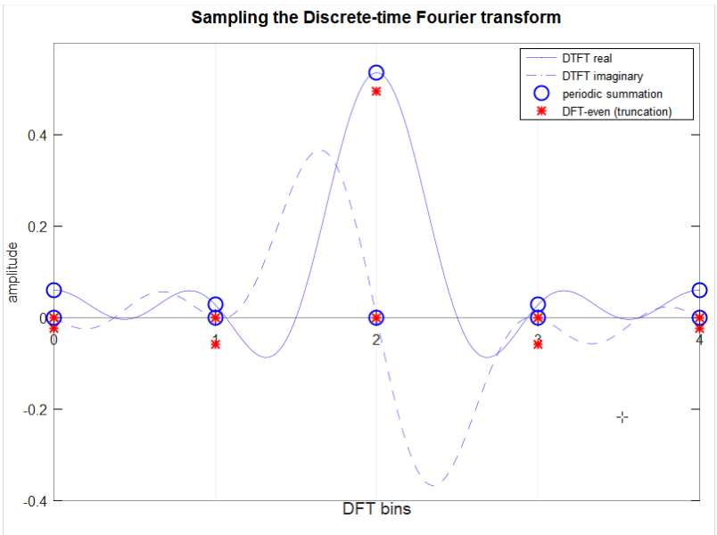
A sampled Fourier transform introduces the frequency viewpoint behind Carleson’s theorem; the Lean project formalizes the precise convergence argument.
Bob K / Wikimedia Commons. Unchanged original image. · Image source · CC0 1.0

Fourier series promise to reconstruct a signal from waves. The subtle question is what reconstruction means: a small average error does not automatically imply convergence at each individual point. A collaborative Lean project makes a major theorem in this territory available as a formal proof. Its explanatory preprint, Formalizing Carleson’s Theorem in Lean, appeared on September 25, 2026; the project itself was completed in July 2025. The formal development proves a generalized Carleson estimate on suitable metric measure spaces and derives a classical corollary for continuous periodic functions. That last restriction deserves attention. Carleson’s original mathematical theorem covers square-integrable functions, while the specific classical corollary highlighted in this formalization assumes continuity. Understanding that distinction reveals the value of exact statements: computer verification becomes informative when a reader can see precisely which theorem was checked.
What a partial Fourier sum remembers
For a function repeating every 2π units, its Fourier coefficients measure how strongly it correlates with oscillations at integer frequencies. A partial Fourier sum keeps only the frequencies from minus N through N. Increasing N adds finer oscillations, but nothing in that definition alone proves that the resulting sequence settles down. The coefficients come from integrals over the whole period; the reconstruction is evaluated at a particular point. The theorem must connect these global measurements with local behavior.
An original easy example is f(x) = 2 plus 3 cos(x) minus sin(2x). Once N reaches two, the partial sum contains every frequency used in f, so reconstruction is exact everywhere. That finite example explains the mechanism but avoids the hard issue. A general continuous function need not have a finite frequency expansion, and the infinitely many remaining coefficients may interact rather than contribute independently. Numerical agreement for the first few thousand terms cannot establish a claim about all later partial sums.
Average, pointwise, and uniform are different promises
Mean-square convergence says that the integral of the squared error tends to zero. Pointwise convergence says that for a fixed location, the error there tends to zero. Uniform convergence requires one index after which the error is small at every location at once. These are different arrangements of quantifiers and different ways to measure failure. A result proved in one mode cannot simply be relabeled as another because a plotted approximation looks convincing.
For a concrete illustration on the unit interval, let g_n be one on the interval from zero to 1/n and zero elsewhere. Its squared integral is 1/n, so its mean-square size tends to zero. Yet its value at zero remains one if the endpoint is included. The example is not a sequence of Fourier partial sums and proves nothing against Carleson’s theorem. Its purpose is to exhibit exactly why a vanishing integral can coexist with failure at an exceptional point, making the stronger reconstruction question mathematically meaningful.
Almost everywhere is a precise kind of smallness
Almost-everywhere convergence permits an exceptional set of Lebesgue measure zero. It does not mean that each exceptional point occurs with a tiny independent probability, nor does it mean that a finite number of pixels may be ignored. A countable set such as the rational points has measure zero despite being dense: every interval contains some of its points. Conversely, a set can be visually hard to recognize while carrying positive measure. Measure, density, and cardinality answer different questions.
One can see why every countable collection is negligible by enumerating its points. Given a positive tolerance ε, cover the first point by an interval of length ε/4, the second by ε/8, and so on. The total length is at most ε/2. Since ε can be arbitrarily small, the points have measure zero. This explanatory construction does not identify the exceptional set of a given Fourier series; it clarifies the mathematical meaning of allowing one. A theorem valid almost everywhere remains a strong statement even when it makes no promise at a chosen exceptional location.
Why the proof studies the worst partial behavior
A typical route toward convergence is to control an operator that measures the largest oscillatory contribution across a family of truncations or frequencies. The supremum brings all those possibilities into one object. A bound on that maximal object can limit the size of the region where troublesome behavior occurs. The metric-space result formalized in this project is a restricted weak-type estimate, with explicit assumptions on the space, the integration kernel, and the collection of modulation functions. Those conditions cannot be discarded merely because the theorem has an abstract title.
A simple independent analogy is the inequality that bounds the measure of points where a nonnegative function h exceeds t by its integral divided by t. On that region, h is at least t, so the integral must be at least t times the region’s measure. The idea converts an integral estimate into a size bound on exceptional behavior. Carleson theory requires much richer machinery to obtain the right estimates, but this elementary argument explains why bounds on operators, rather than direct inspection of every point, can lead to convergence statements.
The geometric assumption called doubling can be illustrated without Fourier analysis. On the ordinary real line with length as measure, a ball of radius r is an interval of length 2r. Doubling its radius produces length 4r, so the measure grows by a factor of two. In the plane with area measure, the corresponding factor is four. An abstract doubling condition requires a controlled growth factor even when the space lacks ordinary coordinates. It does not automatically guarantee the theorem: the kernel and modulation assumptions still have to hold. The example explains one hypothesis, not the entire generalized result.
Equal almost everywhere does not mean equal at a point
In integration theory, functions that differ only on a measure-zero set often represent the same element of an Lp space. That identification is useful because integrals and norms cannot distinguish those changes. Evaluating at a particular point, however, can distinguish them immediately. If f is zero everywhere and g is one at zero but zero elsewhere, their integrals and Lp distance agree with those of identical functions, yet f(0) and g(0) differ.
This creates a practical choice in formal mathematics. Work with an actual function together with evidence that it belongs to the desired space, or work with a quotient object that already identifies functions equal almost everywhere. The project’s exposition discusses that tradeoff and the bookkeeping it creates. For readers, the lesson is that apparently harmless notation can hide a representation choice. A statement involving a point value needs a representative or an almost-everywhere formulation; one cannot retrieve pointwise information that a quotient deliberately forgot.
A completed artifact still needs a faithful statement
The project publishes an informal blueprint alongside the formal source. The blueprint organizes the mathematical dependencies, while the code records proofs the checker can verify. The repository also documents how to build the project and inspect the main theorems’ axiom dependencies. That is more informative than treating a compilation screenshot as the entire result. A completed proof should avoid unfinished placeholders in the relevant dependency chain and should establish the intended definitions, not an easier statement accidentally given a familiar name.
The next mathematical benefit may come from reuse: estimates, measure-theoretic interfaces, and operator definitions can support further formal harmonic analysis. That prospect should be distinguished from an accomplished theorem. This article does not claim that every endpoint case, every Lp generalization, or every application has been formalized. The concrete achievement reported in 2026 is an inspectable development completed in 2025, including a broad metric-space estimate and a continuous-function convergence corollary. Its precision makes both the power and the present boundary of the result easier to understand.
Sources & further reading
Primary papers, project documentation, and research releases used in this article. Publication dates below refer to the sources themselves.
- Formalizing Carleson’s Theorem in LeanBecker and collaborators / arXivPublished Checked
- A blueprint for the formalization of Carleson’s theorem on convergence of Fourier series: IntroductionCarleson formalization projectChecked
- Formalization of a generalized Carleson’s theoremCarleson formalization collaborators / GitHubChecked
- Carleson operators on doubling metric measure spacesBecker, van Doorn, Jamneshan, Srivastava, and Thiele / arXivPublished Checked
- AxiomsLean projectChecked
FOLLOW THE QUESTION
Explore mathematics