ARTIFICIAL INTELLIGENCE
Denoising diffusion: how the 2020 model learned to reverse noise
The 2020 DDPM paper made image generation a sequence of learned denoising steps. Its noise equation and experiments clarify what was new and what came later.
Research checked
Newest cited publication
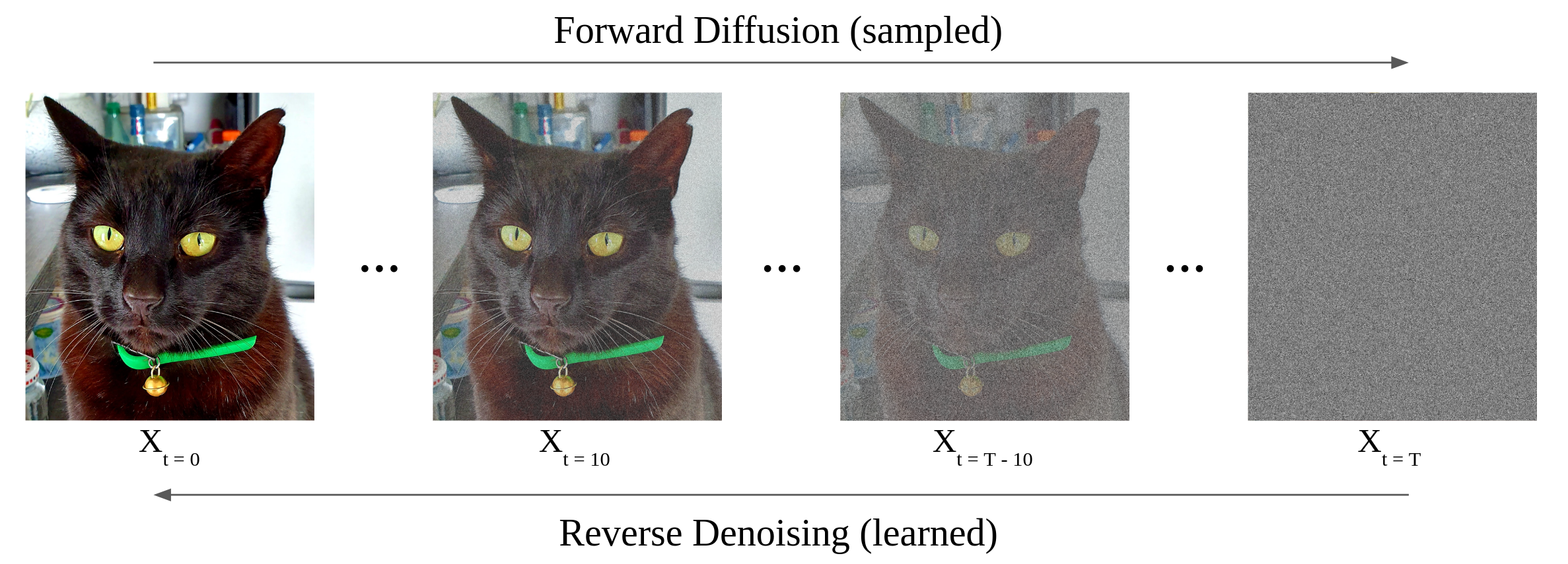
A modern diffusion-process illustration contrasts sampled forward corruption with a learned reverse process. The reverse arrow represents generative denoising, without promising exact recovery of the pictured original.
Dragweb / Wikimedia Commons. Unmodified original image. · Image source · CC BY-SA 4.0

A noisy image seems to contain less information than a clean one. Denoising diffusion probabilistic models use that destruction as a training resource. Jonathan Ho, Ajay Jain, and Pieter Abbeel's June 2020 paper showed how a network could learn many small denoising tasks and then compose them into image generation. The surprise was not that adding noise is reversible for an individual photograph. It generally is not. The model instead learns a distribution of plausible reverse transitions. That distinction explains both the method's power and the care required when calling its outputs reconstructions.
The forward-and-reverse idea predates 2020
Jascha Sohl-Dickstein and colleagues' March 2015 work introduced a generative framework that gradually corrupts data and learns a reverse process. Ho and colleagues built on that lineage in 2020, connecting diffusion training with denoising-based learning and demonstrating much stronger image synthesis. The abbreviation DDPM names their denoising diffusion probabilistic model approach; it should not erase the earlier formulation.
One analogy is learning how to organize increasingly messy collections of colored tiles. At mild disorder, the task is mostly local correction. At severe disorder, several arrangements could fit what remains. Training at many disorder levels gives the learner a family of conditional tasks. Starting from a very disordered arrangement and applying those learned corrections can create a new coherent pattern. The analogy has limits: image diffusion uses a specified stochastic corruption process and a probabilistic model, rather than a person sorting tiles according to a remembered picture.
Signal and noise are balanced through their variances
In the Gaussian formulation, a corrupted image at time t can be written as a signal-scaled clean image plus independent Gaussian noise. If a denotes the product of all signal-retention factors up to that step, the coefficients are square root of a for the image and square root of one minus a for the noise. This gives direct access to a chosen corruption level without simulating every preceding step during training.
For example, set a to 0.64. The signal coefficient is 0.8 and the noise coefficient is 0.6. If a scalar clean-data component has zero mean and variance one, and independent noise also has variance one, the mixture's variance is 0.8 squared plus 0.6 squared, which equals one. The amplitudes do not sum to one; their squared contributions do. This distinction prevents a common misunderstanding about the schedule. Retaining a fixed overall scale can coexist with steadily losing information about which clean example was present.
The training target is noise the experimenter created
Training draws a clean example, a noise level, and random noise. A network receives the resulting corrupted input and the time indicator, then predicts the injected noise. The simplified objective compares prediction with the known noise using squared error. Supervision comes from the corruption procedure, so the experimenter does not need a separately photographed noisy counterpart for every clean training image.
A scalar exercise makes the target concrete. Let the clean value be 0.5 and the sampled noise be minus one. Using the previous coefficients gives an observed value of 0.8 times 0.5 plus 0.6 times minus one, or minus 0.2. If the network predicts minus 0.8 for the noise, its squared prediction error is 0.04. That does not mean it has identified the unique original clean value. Other clean-noise combinations can produce the same observation. Across many examples, squared-error learning favors a conditional average, which must then be used within the specified reverse-process equations.
Generation samples possibilities rather than recovering a secret
At generation time, the process begins with a Gaussian draw and repeatedly applies learned reverse transitions. In the original DDPM setup, the transitions include prescribed stochasticity rather than simply subtracting one predicted noise image and declaring the task finished. The time-dependent coefficients connect those steps to the forward construction.
Imagine two distinct clean patterns that become hard to distinguish under heavy corruption. A single noisy observation cannot reliably tell an algorithm which pattern produced it. A generative model should represent plausible possibilities instead of inventing certainty about the past. This is why a generated sample is not evidence that a matching scene once existed in the world. It also explains why starting from fresh noise can work: the goal is to reach a sample from the learned image distribution, rather than retrieve a training photograph whose identity was hidden in the initial noise. The procedure relies on learned statistical structure and approximation quality, not an inversion miracle.
What the paper actually demonstrated
The 2020 paper reported unconditional image generation on CIFAR-10 and higher-resolution image datasets. Its best reported CIFAR-10 Fréchet Inception Distance, abbreviated FID, was 3.17 under its training-set reference protocol. FID compares distributions of learned image features; it is not a percentage of correct pictures. The paper also reports a different value when using the test-set reference, illustrating why the evaluation protocol matters.
Its experiments used a thousand diffusion steps and a time-conditioned neural backbone. These details belong to this historical configuration, rather than every later diffusion application. A fair reproduction would preserve the dataset split, preprocessing, sampling procedure, and feature-evaluation pipeline. Changing the reference population can move a score without changing a single generated image. Conversely, a favorable aggregate score can coexist with recurring local defects. The result established a strong image-generation approach under stated conditions, not general correctness across arbitrary subjects or a finished text-directed creative system.
DDIM separated a training objective from a sampling path
Jiaming Song, Chenlin Meng, and Stefano Ermon introduced denoising diffusion implicit models, or DDIMs, in October 2020. Their work constructs a family of processes compatible with the same training objective while enabling different, faster sampling procedures. This was a separate contribution after the June DDPM paper. Its reported acceleration should not be attributed to the original thousand-step experiment.
An engineering question follows: how much quality is lost when a sampler uses fewer network evaluations? The answer needs a curve rather than one promotional number. Measure generation time and several quality diagnostics over increasing evaluation budgets while keeping the trained model fixed. This separates improvements in the sampler from improvements in training. It also exposes a practical tradeoff: a slow process may be acceptable for an offline artifact but unsuitable for an interactive tool. Different routes through the learned representation can make that same model useful in different settings.
Denoising skill is not universal knowledge
The authors' released implementation makes the original procedures inspectable, including how noise schedules and reverse transitions are represented. This matters historically because the method is more specific than an animation of static gradually becoming a picture. Reproducing its assumptions helps distinguish a learned probabilistic model from a suggestive visualization.
For a diagnostic, train on simple patterns with known component frequencies, reserve some combinations for evaluation, and inspect both the outputs and how their frequencies change. Check whether rare patterns disappear, whether near-copies recur, and whether performance deteriorates when the sampling budget changes. A network can become good at the training distribution without understanding the physical or semantic meaning of its outputs. The enduring contribution of DDPM is a tractable learning construction that turns deliberately corrupted data into useful generative supervision. Its boundaries remain experimentally accessible: ask which distributions it captures, at what computational cost, and under which sampling and evaluation rules.
Sources & further reading
Primary papers, project documentation, and research releases used in this article. Publication dates below refer to the sources themselves.
- Denoising Diffusion Probabilistic ModelsarXivPublished Checked
- Deep Unsupervised Learning using Nonequilibrium ThermodynamicsarXivPublished Checked
- Denoising Diffusion Implicit ModelsarXivPublished Checked
- diffusion_utils.pyJonathan HoChecked
FOLLOW THE QUESTION
Study engineering foundations