ARTIFICIAL INTELLIGENCE
Generative adversarial networks: the 2014 game that changed image synthesis
The original GAN paper turned generation into a learned competition. Its equations, early experiments, and later revisions reveal both the insight and its limits.
Research checked
Newest cited publication
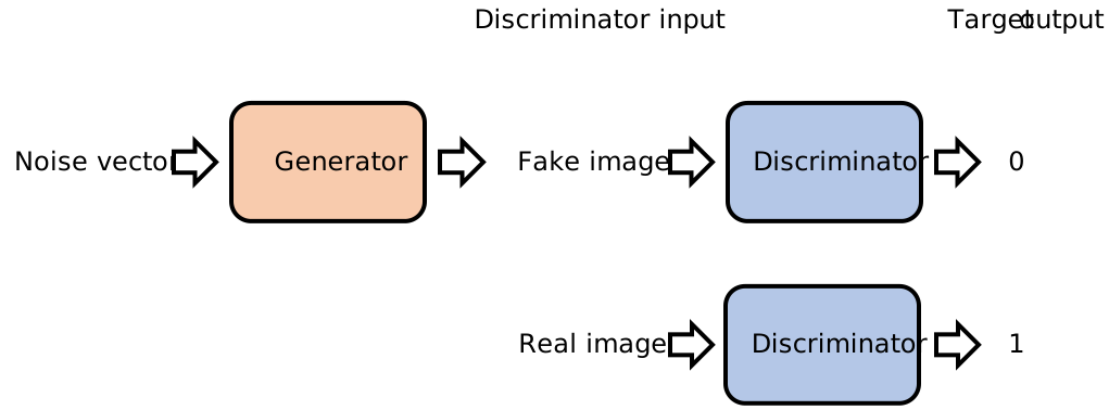
A later GAN schematic shows real and generated inputs passing through a shared discriminator. The two drawings represent the same discriminator; the zero and one labels express its training targets.
Mtanti; Basque translation by Ksarasola / Wikimedia Commons. Unmodified downloaded SVG. · Image source · CC BY-SA 4.0

In June 2014, Ian Goodfellow and colleagues proposed training a generator with feedback from another learned model. The generator would produce examples, and a discriminator would distinguish them from training data. This adversarial arrangement supplied a way to learn a complicated distribution without first writing down its probability density. Looking back from October 2026, the landmark is easier to understand by separating the original mathematical idea from the impressive image systems that came later. The 2014 paper offered a productive game, rather than a guarantee that any two neural networks would learn to play it well.
A generator needs a useful opponent
A generative adversarial network, or GAN, contains two differentiable functions. The generator maps a random input to a candidate example. The discriminator assigns that example a probability of belonging to the real-data source. During alternating updates, the discriminator improves its classification, while the generator changes its output to receive a more favorable response. The learned evaluator supplies feedback that a fixed pixel-comparison rule would miss.
Consider a simple task: create small drawings of chairs. Comparing each generated drawing with one randomly selected training chair would punish valid differences in viewpoint or shape. An evaluator trained across many examples can instead learn recurring regularities. This does not make its judgment objective. If the dataset mostly contains front-facing chairs, the evaluator may reward that narrow convention. The game transfers the definition of convincing from a hand-written distance to a learned decision boundary, with all the advantages and blind spots that learning introduces.
The discriminator estimates a density ratio
The original analysis studies an ideal discriminator with enough capacity and exact optimization. With equal prior odds for real and generated examples, its optimal output at an observation x is the real probability density divided by the sum of real and generated densities. Where those distributions agree and have support, that output is one half. This is a statement about the ideal game, not a certificate issued by an ordinary classifier with fifty-percent accuracy.
Consider a discrete calculation. Suppose real examples are type A three quarters of the time and type B one quarter, while the generator emits each type equally often. For type A, the optimal real-source probability is 0.75 divided by 1.25, or 0.6. For type B, it is 0.25 divided by 0.75, or one third. Equal generation frequencies therefore do not fool the ideal discriminator. If the generator eventually matches the three-to-one mixture, both source probabilities become one half. The relevant achievement is matching frequencies as well as making individual examples look plausible.
An equilibrium is not an optimization recipe
The original theorem considers distributions and ideal function spaces. Actual training moves a finite set of neural-network parameters using noisy gradient estimates. Both players change, so each faces a moving objective. A useful best response can become obsolete after the opponent updates. Small training losses alone therefore cannot establish that the model has reached the distributional solution described by the theorem.
A simple classroom game makes this difference visible. Let a generator choose between two drawing styles, and let an evaluator specialize in spotting whichever style appeared most recently. The generator can keep switching styles without learning the full distribution. Changing the update schedule can change the motion of the game even when neither network changes size. This is why a convergence claim needs its assumptions spelled out. More capacity may strengthen the evaluator while making its feedback harder for a weak generator to use. The question is whether the interaction supplies a helpful direction, not merely whether each participant can fit its own immediate training examples.
The first demonstrations were a beginning
The 2014 paper demonstrated the approach on handwritten digits, faces, and small natural images. Its quantitative comparisons included density estimates built from generated samples using Parzen windows, a smoothing method. Those evaluations belong to their historical setting. They should not be read as measurements from a modern high-resolution text-to-image system, or as direct access to the generator's exact likelihood.
In November 2015, Alec Radford, Luke Metz, and Soumith Chintala introduced deep convolutional GANs, usually called DCGANs. Their paper investigated architectural choices and learned visual representations. This later work helped turn the adversarial idea into a more practical image-learning approach, but it was a separate contribution. Historical accounts lose explanatory power when the original game, later convolutional designs, and subsequent high-resolution results are compressed into one discovery. Distinguishing them reveals how progress depended on experiments that made an appealing principle train more reliably.
Wasserstein GAN changed the question being optimized
Martin Arjovsky, Soumith Chintala, and Léon Bottou's January 2017 Wasserstein GAN paper examined how the distance between distributions affects learning. Its critic estimates a transport-related objective under a smoothness constraint, rather than acting as the original probability-valued real-versus-generated classifier. This is a later reformulation, not the loss function introduced in 2014.
A one-dimensional example explains the attraction of transport. Put all real probability at position zero and all generated probability at position three. Moving the generated mass to position two is geometrically useful: the transport distance drops from three to two. A perfect binary classifier can still distinguish the two sources in either case. Its certainty alone does not reveal how far apart they are. The example does not prove that a finite neural critic learns the correct distance. It shows why the geometry of the objective can matter as much as the expressive power of the generator.
A convincing sample can conceal a missing population
Lucas Theis, Aäron van den Oord, and Matthias Bethge's November 2015 evaluation paper explains why visual fidelity, likelihood, and sample-based density estimates need not agree in high dimensions. The lesson is especially relevant to adversarial generation: a gallery can demonstrate that plausible examples exist without measuring how much of the target distribution the generator covers.
For a simple test, define four equally common categories of simple shapes. A generator that produces only excellent circles covers one category while missing the other three. Increasing the number of circle samples does not repair that omission. An evaluator should therefore measure category frequencies, within-category variation, and fidelity separately. Real image distributions rarely provide such clean labels, making the problem harder. Nearest-neighbor inspection can flag obvious copying, but the absence of a close match in one representation is not a proof against memorization. Different diagnostics answer different questions, and a strong report makes those distinctions visible.
The enduring insight is a learned comparison
The GAN framework made a discriminator useful as more than a final classifier: its behavior could shape the examples another network learned to produce. That is the historical mechanism worth preserving. The original construction did not require that every future generator use the same architecture, and later revisions explored what happened when the evaluator, objective, or data representation changed.
A reproduction exercise can retain this insight without pursuing photorealism. Generate two-dimensional point clouds with known component frequencies, log both players' updates, and compare repeated runs. A scatterplot exposes omitted clusters that a single average loss can hide. Freeze the evaluator occasionally and test it on deliberately flawed outputs to learn what it has actually noticed. Such an experiment connects the elegant ideal solution with the messy dynamics that determine whether training reaches anything useful. The landmark remains valuable precisely because its promise and its failure modes can both be studied in a small, transparent system.
Sources & further reading
Primary papers, project documentation, and research releases used in this article. Publication dates below refer to the sources themselves.
- Generative Adversarial NetworksarXivPublished Checked
- Unsupervised Representation Learning with Deep Convolutional Generative Adversarial NetworksarXivPublished Checked
- Wasserstein GANarXivPublished Checked
- A note on the evaluation of generative modelsarXivPublished Checked
- NIPS 2016 Tutorial: Generative Adversarial NetworksarXivPublished Checked
FOLLOW THE QUESTION
Study engineering foundations