MATHEMATICS
When a Random Matrix’s Geometry Survives at the Spectral Edge
A 2026 preprint compares spectral edges through variance-profile random walks, explaining why structured randomness can retain its geometry at large size.
Research checked
Newest cited publication
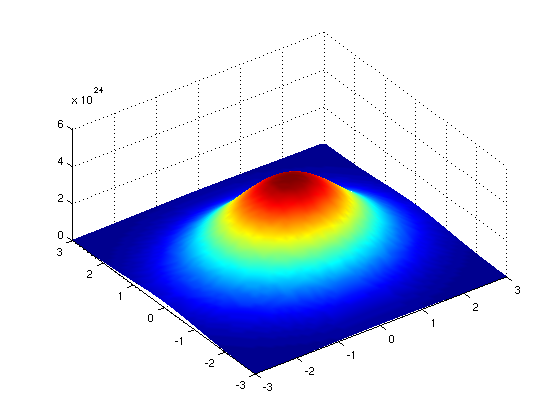
A Gaussian surface provides familiar probabilistic background for a discussion of random matrices with structured variance profiles.
Michael Hardy / Wikimedia Commons. Unchanged original image. · Image source · Public domain (released by the creator)

The largest eigenvalue of a random matrix looks like a single number, but it can remember how randomness was distributed across thousands of entries. A dense matrix lets nearly every coordinate interact with every other coordinate. A band matrix allows mainly nearby interactions. Both may have centered entries and the same total variance in each row, yet their extreme eigenvalues need not fluctuate in the same way. A preprint first submitted by Dang-Zheng Liu and Guangyi Zou on 22 April 2026 studies this difference through an unexpected intermediary: a Markov chain built from the entry variances. Its perspective makes universality a question about geometry and transport, rather than a promise that every sufficiently large random object behaves alike.
The new result compares structures, with conditions
The 2026 paper, Edge Universality for Inhomogeneous Random Matrices II: Markov Chain Comparison and Critical Statistics, develops quantitative comparison conditions for symmetric or Hermitian matrices. Independence holds up to the required symmetry. The squared variance amplitudes form a symmetric Markov transition matrix; the entries also satisfy specified symmetry and moment bounds. Under additional bounds on return probabilities, cumulative comparison errors, sparsity and any finite-rank deformation, mixed polynomial trace statistics agree asymptotically between two models. This provides a route to matching spectral-edge laws in critical and subcritical regimes.
That is a preprint theorem under hypotheses, rather than a statement about arbitrary measured networks. The distinction between matching two structured ensembles and matching a classical Gaussian ensemble matters. Two models can share an edge law that differs from the familiar mean-field answer. The article below uses elementary examples to explain why that possibility is natural; these examples are not new results of the preprint.
A variance table becomes a random walk
Here is a concrete construction. Take twelve matrix coordinates arranged in a circle. In one model, assign variance 1/12 to every entry in a row. In another, assign variance 1/3 to the coordinate itself and its two neighbors, and zero elsewhere. Each row sums to one, and both variance tables are symmetric. Reading a row as a list of transition probabilities defines a random walk: the first walk forgets its starting point after one step, whereas the second moves locally.
After one step the local walk reaches only three coordinates. After two steps it reaches at most five. The two variance tables therefore encode markedly different information even though their row totals agree. Squaring the matrix entry amplitudes is crucial: amplitudes themselves do not generally add to one. This dictionary separates two kinds of randomness. The matrix entries are random coefficients, while the associated walk is a mathematical device whose deterministic transition probabilities describe where those coefficients have substantial variance.
Why traces can detect that motion
For a symmetric matrix H, the trace of H squared is the sum of H(i,j) squared over all ordered pairs. Taking expectations records the total entry variance. This calculation cannot distinguish the two twelve-coordinate examples: both totals equal twelve. Higher powers expose more structure. Expanding the trace of H to the fourth power gives products along closed sequences i to j to k to l to i. Independence and centering eliminate many products when their expectations are taken.
Terms that survive depend on which indices coincide and which variance-weighted paths can close. This is an elementary reason that a walk appears in spectral analysis. The calculation becomes more involved at large powers, and the research uses specialized polynomial traces and diagram estimates. But the basic bookkeeping is visible without those tools: a trace sums loops, expectation assigns weights to loops, and a local variance pattern constrains which loops carry substantial weight. Knowing only the total variance discards this information.
An edge needs a different magnifying glass
Suppose a normalized matrix has about N eigenvalues spread over an interval of constant length. In the middle of a region with positive limiting density, a typical gap has order 1/N. Near a regular square-root edge, the density becomes small. Write the distance below the edge as d. If density is proportional to the square root of d, the expected number of eigenvalues in the final interval of width d is proportional to N times d to the power three halves.
Setting this count equal to one gives d of order N to the power minus two thirds. This is an explanatory scaling calculation, assuming a regular square-root edge; it is not a universal formula for every variance profile. It shows why a proof about middle-of-spectrum spacings cannot simply be moved to the largest eigenvalue. The edge asks about rare extremal behavior on another scale, where transport, spikes and finite-size corrections can become decisive.
What universality is allowed to forget
Imagine replacing each nonzero coefficient in the local twelve-coordinate model by another centered random variable with the same variance. If a suitable theorem applies, fine details such as the exact coefficient histogram may disappear from the limiting answer. The locality pattern, however, remains. Universality can erase the distribution of individual entries while retaining the geometry of the places where entries interact. Treating those two operations as equivalent would erase the central mathematical question.
The earlier Liu–Zou paper, submitted on 25 August 2025, obtained classical real or complex Gaussian edge laws under a short-to-long mixing condition. In contrast, the 2026 continuation investigates comparison when full mean-field behavior is not the appropriate reference. Separately, the local-relaxation-flow work of Erdős, Schlein and Yau established bulk spacing universality for a class of symmetric matrices with subexponential entry tails. These are related milestones with different observables and assumptions, rather than interchangeable versions of one result.
How to test the idea without overclaiming
A useful numerical exploration would hold the row-variance normalization fixed while changing the interaction width. For each size, generate many independent matrices, record the largest eigenvalue, and examine a centered and rescaled distribution. Repeat with two entry distributions that satisfy the relevant moment conditions. Agreement across entry distributions and disagreement across geometric profiles would probe two separate aspects of the theory. A small experiment could reveal a coding mistake or suggest a pattern; it would not establish an asymptotic theorem.
Centering deserves particular attention. A shifting spectral edge can make two otherwise similar fluctuation laws look different, while an unjustified fitted shift can conceal a real correction. Keep the centering rule explicit before comparing histograms. The broader lesson is a practical reading strategy for random-matrix news: identify the observable, the normalization, the symmetry class, the variance geometry and the limiting regime. Only after those choices are fixed does the word universality have a precise mathematical job to do.
A second original calculation makes the danger of disconnected geometry explicit. Form a block diagonal matrix from two independent, identically distributed random blocks. Its largest eigenvalue is the larger of the two block maxima. If each block maximum has cumulative distribution F at a threshold, the full maximum has cumulative probability F squared at that same threshold. At a threshold where F equals one half, that probability is one quarter. This identity is exact for every block size and does not rely on an asymptotic approximation. The variance-profile walk cannot cross between the two blocks, so it has retained a structural obstruction that no change in entry histogram can remove. A comparison theorem’s transport hypotheses are therefore doing real work: they exclude or distinguish geometries whose extremal behavior is altered before any subtle limit is taken. Checking whether the variance graph is connected is therefore a sensible first diagnostic, even though connectivity alone is much weaker than the required quantitative comparison bounds.
Sources & further reading
Primary papers, project documentation, and research releases used in this article. Publication dates below refer to the sources themselves.
- Edge Universality for Inhomogeneous Random Matrices II: Markov Chain Comparison and Critical StatisticsarXivPublished Checked
- Edge Universality for Inhomogeneous Random MatricesarXivPublished Checked
- Universality of Random Matrices and Local Relaxation FlowarXivPublished Checked
FOLLOW THE QUESTION
Explore mathematics