MATHEMATICS
The Last Unvisited Site Is More Than a Coupon Collector
An October 2026 preprint identifies a randomly shifted Gumbel cover-time law for the two-dimensional torus, revealing persistent large-scale correlations.
Research checked
Newest cited publication
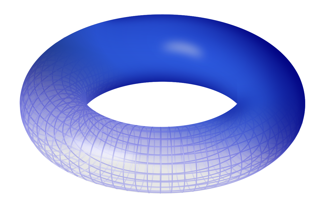
A torus illustrates periodic geometry. The cover-time result concerns a discrete torus and a random walk, rather than motion on this rendered surface.
Leonid 2 / Wikimedia Commons. Wikimedia-generated PNG rendering of the SVG; no editorial changes. · Image source · CC BY-SA 3.0

A random walker can visit almost every location and still take a surprisingly long time to find the final few. On a square grid whose opposite sides are identified, this exploration problem is called the cover time of the two-dimensional discrete torus. The word torus describes the boundary rule: stepping off the right edge brings the walker back at the left. It does not require walking on a doughnut-shaped surface. A preprint submitted by Yechi Zhou on 1 October 2026 identifies a limiting law for the remaining fluctuations after the leading terms are removed. The proposed theorem connects the final unvisited regions to a random Gaussian measure. It is a recent preprint result, and the exact normalization is part of its mathematical content.
Specify the experiment before timing it
Take an N by N periodic grid. At a jump, choose one of the four nearest neighbors with equal probability. In the continuous-time convention used here, the total jump rate is one, so the expected time between jumps is one. The cover time is the first time at which every one of the N squared vertices has been visited. It includes the starting vertex from time zero. Changing the total jump rate changes the time scale, even though the sequence of visited vertices has the same distribution.
For example, a convention assigning rate one to each of the four directions gives total rate four. Under that clock, expected holding times are one quarter as long. A number reported without the clock convention would therefore be ambiguous by a factor of four. This is a general lesson for probability news: a constant can be mathematically meaningful only after the process has been specified. It is especially important when comparing discrete-time steps with continuous-time elapsed time or results stated for different boundary conditions.
From a leading scale to a full limiting law
Dembo, Peres, Rosen and Zeitouni’s work, first posted on 26 July 2001 and published in 2004, established a leading cover-time scale of (4/pi) times N squared times the square of log N. Such a statement predicts the dominant size, but leaves open the distribution of the residual error. A smaller fluctuation can be invisible after division by the leading term and still be much larger than one.
Zhou’s rate-one preprint states that T divided by [(2/pi) N squared log N], minus 2 log N plus log log N, converges in distribution to G + log(kappa Z). Here G is standard Gumbel, Z is the positive total mass of critical Gaussian multiplicative chaos for the zero-average Gaussian free field on the unit torus, G and Z are independent, and kappa is deterministic and positive. All logarithms are natural. The formula retains a random shift, not just a fitted constant.
Why independent sampling is a useful wrong model
An original comparison starts with M equally likely coupons sampled independently. When k distinct types have been collected, the chance that the next draw is new equals (M minus k) divided by M. The mean waiting time for the next discovery is therefore M divided by (M minus k). Adding these waiting times gives an expected total of M times the harmonic sum 1 + 1/2 + ... + 1/M, approximately M log M. The final few coupons dominate the slow tail because their waiting times are longest.
If grid vertices were independent coupons and M equaled N squared, that estimate would have order N squared log N. The actual two-dimensional walk has an additional logarithmic factor at leading order. The comparison fails because consecutive positions are neighbors, returns are common, and unvisited sites are spatially correlated. A walker can spend a long time revisiting one region while another remains untouched. The coupon calculation is still valuable: it isolates the effect of repeated independent attempts, making it easier to recognize the extra geometric obstruction in the real problem.
A mixture remembers earlier randomness
The standard Gumbel distribution has cumulative probability exp(-exp(-x)). If a positive random variable Z is independent of a Gumbel variable G, condition on Z = z. Then the probability that G + log(kappa z) is at most x equals exp(-kappa z exp(-x)). Averaging over Z gives the expectation of that expression. This elementary computation shows exactly how a random shift differs from adding one deterministic offset: different realizations retain different effective amounts of unfinished exploration.
For a toy mixture, let kappa equal one and let Z take values one and four, each with probability one half. At x = 0 the cumulative probability is [exp(-1) + exp(-4)] divided by two, approximately 0.1931. Replacing Z by its mean, 2.5, would instead give exp(-2.5), approximately 0.0821. Averaging the intensity before applying the exponential is not equivalent to averaging afterward. The example does not model the actual Gaussian measure; it illustrates why erasing the random shift changes observable probabilities.
A measure can describe where difficulty accumulates
A random measure assigns a random nonnegative weight to each region, consistently under subdivision. Imagine coloring a large grid by how difficult different regions are to finish exploring. The total weight is one summary of that map, while normalized regional weights describe relative locations. A Gaussian free field is a correlated Gaussian object associated with the geometry; multiplicative chaos is a carefully normalized random measure built from such a field. At criticality, ordinary exponentiation is insufficient without the appropriate limiting normalization.
A related 2026 result has a different boundary rule. In a preprint submitted on 24 February, Oren Louidor and Santiago Saglietti obtain a joint cover-time and last-visited-location limit for lattice approximations of planar domains with wired boundaries. Their limiting location is governed by a normalized critical Liouville measure. This comparison explains why identifying a total mass is informative without identifying every spatial detail. It also warns against transplanting a wired-domain theorem to a periodic grid: identifying boundary vertices and wrapping opposite sides produce different processes and require separate arguments.
Separate centering from evidence for a law
A numerical study should record many independent cover times for several grid sizes, retain the stated jump convention, and apply a prespecified centering and scaling. Fitting a separate shift for every size can make unrelated distributions look deceptively similar. The logarithmic correction also decays slowly relative to the main term, so moderate sizes may be dominated by finite-size effects. Reporting a histogram without the normalization and sample count would conceal more than it explains.
The preprint’s proof strategy separates the number of small unvisited components before coverage from their disappearance in the final window. The central conceptual point is broader than a particular proof: exploration inherits randomness from both the spatial pattern left behind and the final waiting times. The October result asserts a precise asymptotic description of that combination. It does not turn a finite simulation into verification of a 203-page proof, and it does not say that every graph has the same cover-time distribution. Geometry remains present even at the final site.
Even the leading scale gives a useful numerical diagnostic. Doubling N multiplies N squared by four, but it also changes the logarithm. The leading-time ratio is four times [log(2N) divided by log N] squared, rather than exactly four. At N = 100 this ratio is about 5.29. The discrepancy is large enough to matter in a small simulation, before the second-order correction is considered at all. These numbers are a calculation from the leading expression, not estimates of actual finite-grid mean cover times. A careful notebook would show both the raw timings and each transformation, so a visual agreement could be traced to an explicit mathematical prediction.
Sources & further reading
Primary papers, project documentation, and research releases used in this article. Publication dates below refer to the sources themselves.
- A limit law for the cover time of the two-dimensional discrete torusarXivPublished Checked
- A Limit in Law for the Cover Time and Last Visited Vertex of Wired Planar DomainsarXivPublished Checked
- Cover Times for Brownian Motion and Random Walks in Two DimensionsarXivPublished Checked
FOLLOW THE QUESTION
Explore mathematics