PHYSICS
Super-Kamiokande’s 1998 Neutrino Result: Reading the Earth as an Oscillation Baseline
How atmospheric neutrinos, Cherenkov rings and an up–down comparison established flavour change in 1998 without measuring individual absolute masses.
Research checked
Newest cited publication
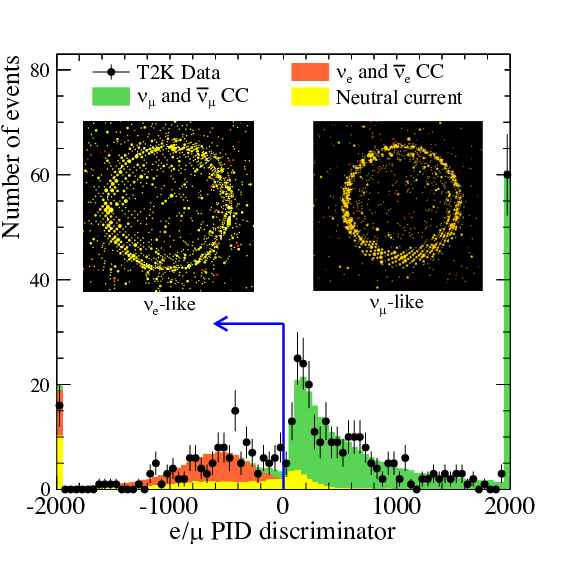
A later T2K figure illustrates electron-like and muon-like Cherenkov-ring classification at Super-Kamiokande. The 2019 explanatory figure provides detection-method context for the separate 1998 atmospheric-neutrino result.
T2K Collaboration, arXiv:1910.03887, Figure 2 · Image source · CC BY 4.0

In 1998, Super-Kamiokande found that the direction from which an atmospheric neutrino arrived mattered in a remarkable way. Muon-neutrino-like events were depleted when the neutrinos had travelled long distances through Earth, while the electron-like sample did not show a comparable pattern. The collaboration announced its evidence on June 5 and posted the landmark analysis on July 3. The result supported neutrino oscillations: a particle created in one flavour could later interact as another. It also implied nonzero neutrino masses within the oscillation framework. This was not a direct weighing of individual neutrinos, nor a complete census of their possible destination flavours. Its strength lay in a controlled comparison across a naturally enormous range of travel distances.
The atmosphere supplied the particles
Cosmic rays striking the upper atmosphere create cascades that include pions and muons. Their decays produce muon-flavour and electron-flavour neutrinos and antineutrinos. A simple pion–muon decay chain suggests roughly two muon-flavour neutrinos for each electron-flavour neutrino, although a real flux calculation must include energy, direction, particle decays and atmospheric conditions. The detector’s event ratio is not simply that production ratio: interaction probabilities and selection efficiencies also matter.
Before the directional discovery paper, Super-Kamiokande had already reported an unexpectedly small muon-to-electron event ratio in a March 1998 preprint. Its measured double ratio, comparing the data’s muon/electron ratio with a simulation’s ratio, was about 0.61. A double ratio reduces some common normalization uncertainties but does not eliminate modeling or classification errors. It also does not mean that exactly 61 percent of every atmospheric muon-neutrino population survived. The selected energies, final states and reference electron sample all enter that interpretation.
Invisible neutrinos became visible through secondary particles
Super-Kamiokande uses a large volume of water to observe rare neutrino interactions. An interaction can produce an energetic electron or muon, whose Cherenkov light forms a ring pattern on the surrounding photosensors. Cherenkov emission occurs when a charged particle moves faster than light travels through water; it does not require exceeding light’s speed in vacuum. The recorded timing and light pattern help reconstruct the event’s position, direction and visible energy.
Electrons initiate electromagnetic showers, producing fuzzier ring boundaries. Muons generally make cleaner, sharper rings. These differences permit electron-like and muon-like classification, rather than a detector literally reading a neutrino flavour label. The analysis must quantify confusion between categories and backgrounds from other interactions. The landmark paper used a 22.5-kilotonne fiducial volume inside the larger tank. Multiplying 22.5 kilotonnes by 535 days and dividing by 365.25 days per year gives about 32.96 kilotonne-years, consistent with the paper’s rounded 33.0-kilotonne-year exposure.
Upward and downward arrivals had different journeys
A downward-going atmospheric neutrino can be created only about 15 kilometres above the detector. A vertically upward-going one may have crossed roughly 13,000 kilometres from the far side of Earth. The outgoing charged particle provides an estimate of the neutrino’s direction, with a resolution that depends on energy and interaction kinematics. Zenith angle therefore acts as a proxy for baseline, the distance over which the neutrino state evolves.
At suitable energies, the no-oscillation expectation is approximately symmetric between upward and downward arrivals. That makes the comparison more discriminating than an overall shortage of events. An uncertain total atmospheric-neutrino production rate would affect many directions together. It would not naturally produce the observed direction-dependent muon-like deficit while leaving the electron-like distribution comparatively unchanged. The experiment still needed flux, cross-section and detector studies, but the directional pattern narrowed the explanations those uncertainties could plausibly support.
Oscillation depends on distance divided by energy
In a two-flavour vacuum approximation, a neutrino’s survival probability is one minus sin²(2θ) multiplied by sin²(1.27 Δm² L/E), when the squared-mass difference is in eV², the distance in kilometres and the energy in gigaelectronvolts. The angle θ describes mixing between flavour states and mass states. The relative quantum phases evolve during travel, changing the probability of detecting a chosen flavour. The probability oscillates; an individual neutrino is not repeatedly inspected during its journey.
For illustration, take maximal mixing and a squared-mass difference of 0.0025 eV². At an energy of one GeV and a distance of 15 kilometres, the phase is about 0.0476 radians and the survival probability about 0.998. The first disappearance minimum occurs near L/E = 495 kilometres per GeV. These chosen values illustrate the scale and are not a replacement for the 1998 fit. Real data average over broad energies, directions and reconstruction errors, which can wash out rapid oscillations into a smoother depletion.
What the 1998 analysis established
The 535-day analysis found a zenith-dependent muon-neutrino deficit incompatible with its no-oscillation expectations after the tested experimental and flux uncertainties were considered. It was consistent with strong two-flavour mixing and a small squared-mass separation. The contemporary June 5 release explicitly allowed muon neutrinos to disappear into undetected tau neutrinos or another possibility, such as sterile neutrinos. That historical qualification matters: the disappearance pattern itself did not identify every missing particle as a detected tau neutrino.
Several logically different statements must remain distinct. A deficit establishes a discrepancy with a reference prediction. Its energy and directional structure tests possible mechanisms. Interpreting that structure as oscillation connects it to mass-state mixing. Separately detecting the destination flavour asks a further experimental question. The 1998 result made a compelling oscillation case because these observations fit a coherent pattern, not because all later neutrino knowledge had already been contained in the first analysis.
The result did not determine the absolute mass scale
Oscillation phases depend on differences between squared masses. Adding the same constant to all squared masses leaves those differences unchanged. Consequently, even a very accurate oscillation measurement cannot by itself specify every absolute mass. The June 1998 release stated that the experiment did not directly determine the masses responsible for the effect. Nonzero squared-mass separation requires at least one nonzero mass, but it does not establish a unique common mass scale or a complete ordering of three states.
This is a useful example of extracting a strong conclusion from incomplete information. Measuring relative heights between floors demonstrates that a building has vertical structure, even without knowing its elevation above sea level. The missing common reference does not weaken the measured differences. Laboratory decay measurements, cosmological observations and other neutrino experiments ask complementary questions about that reference and the larger mixing framework. Their future information should be combined with the oscillation evidence through the appropriate physical model.
The later L/E test strengthened the mechanism
In April 2004, the collaboration posted a separate analysis that found a dip in the distribution of travel distance divided by neutrino energy, as expected from an oscillatory transition probability. This was later evidence with its own event selection and data, not a feature to attribute retrospectively to the original 1998 sample. Resolving a dip is more demanding than observing a broad deficit because poor distance or energy reconstruction can blur the characteristic structure.
The progression shows why the 1998 discovery was a beginning rather than a completed neutrino theory. An atmospheric anomaly became a direction-dependent disappearance signal, and improved measurements then tested the shape expected from quantum interference. The lasting achievement was to turn Earth’s size into an experimental resource: the same detector could compare short and long neutrino journeys. Careful reconstruction and comparisons revealed a change in flavour that a total count alone would have made much harder to establish.
Sources & further reading
Primary papers, project documentation, and research releases used in this article. Publication dates below refer to the sources themselves.
- Evidence for oscillation of atmospheric neutrinosSuper-Kamiokande Collaboration / arXiv; Physical Review LettersPublished Checked
- Measurement of a small atmospheric νμ/νe ratioSuper-Kamiokande Collaboration / arXiv; Physics Letters BPublished Checked
- Official Super-Kamiokande Press Release from JapanSuper-Kamiokande Collaboration / University of Hawaii archivePublished Checked
- Evidence for an oscillatory signature in atmospheric neutrino oscillationSuper-Kamiokande Collaboration / arXiv; Physical Review LettersPublished Checked
FOLLOW THE QUESTION
Explore physics