PHYSICS
Reading Sagittarius A* flares in two infrared colors
Webb’s paired infrared light curves and a 2026 multiwavelength analysis reveal how timing can test competing explanations for Sagittarius A* flares.
Research checked
Newest cited publication
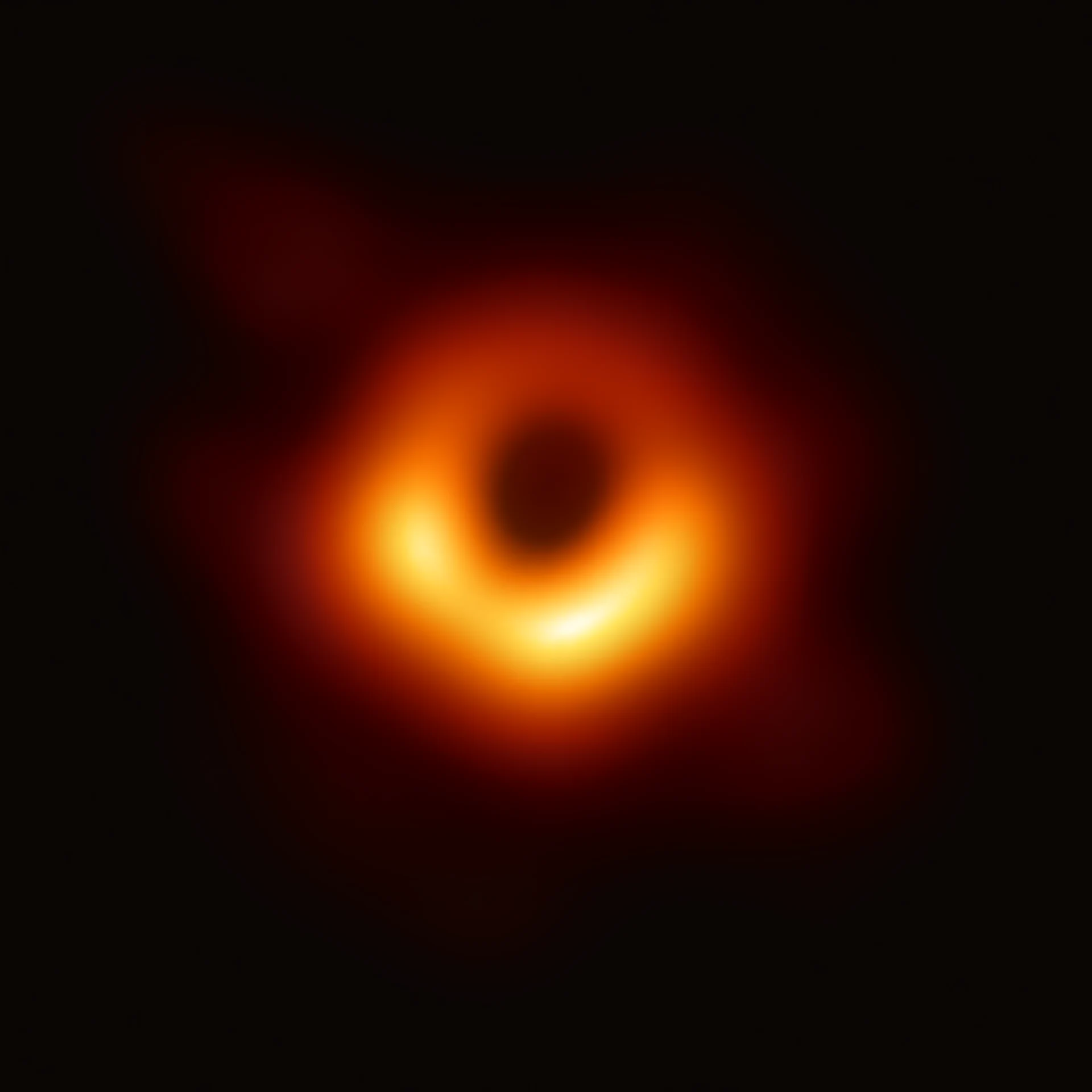
The M87 black-hole image supplies observational context. Sagittarius A* is a separate Galactic-center source whose infrared flares are measured by a different method.
Event Horizon Telescope / ESO · Image source · CC BY 4.0

The Milky Way’s central black hole is difficult to watch as a changing object. Nearby stars crowd the view, dust blocks visible light, and the emitting region changes rapidly. Webb observations reported in February 2025 opened a useful channel: uninterrupted stretches measured in two infrared bands at once. A simultaneous infrared, X-ray, and radio study, revised in February 2026, expands that timing experiment. The central question is not whether Sagittarius A* flickers. It is whether the order, color, and duration of its flickers can tell us how electrons acquire and lose energy. A light curve can contain physical information that a single beautiful image cannot provide.
Two colors sharing one clock
The first study used approximately forty-eight hours of simultaneous observations at wavelengths of 2.1 and 4.8 micrometers, distributed across seven epochs in 2023 and 2024. It found continuing variability, different behavior in faint and bright emission, and a short delay of the longer-wavelength signal relative to the shorter-wavelength signal. The paper appeared on arXiv in January 2025; NASA’s February 18 release identifies the publication in The Astrophysical Journal Letters that day.
Simultaneity is essential. Suppose an astronomical source brightens and fades in ten minutes. Measuring one color before the peak and a second color after it could manufacture an apparent spectral difference even if the source’s intrinsic color stayed fixed. Simultaneous measurements avoid this particular ambiguity by assigning each pair of brightness values to the same time. Remaining differences can then be tested against detector noise, calibration, and real physical evolution.
A color measurement need not look like an ordinary red or blue photograph. Here it is a ratio or relationship between brightnesses in two infrared bands. When that relationship changes during a flare, the spectrum is evolving. When it retraces a different path while fading than while rising, a single brightness value no longer uniquely identifies the source’s physical state. The observation begins to constrain the history of the particles producing the radiation.
How energetic electrons turn time into color
Charged particles moving through magnetic fields can produce synchrotron radiation. For an electron moving relativistically, a characteristic radiation frequency scales approximately with magnetic-field strength times the square of the electron’s Lorentz factor. The Lorentz factor describes how relativistic the electron is. At fixed field strength, higher-frequency synchrotron emission generally selects more energetic electrons. This makes color a possible probe of the particle population rather than a decorative property of the source.
The same particles lose energy by radiating. In a simple synchrotron-dominated model, the cooling time decreases as magnetic-field strength squared and particle energy increase. Combining these scalings shows why higher-frequency emission can fade sooner. For an illustrative fixed field, increasing observing frequency by a factor of four selects electrons with roughly twice the Lorentz factor and approximately half the cooling time. That example is a scaling exercise, not a measurement of Sagittarius A*’s field.
The 2025 authors modeled an evolving electron population and found that synchrotron evolution could reproduce important light-curve features. Their inferred field strengths depend on that model. Such estimates are not equivalent to inserting a magnetometer into the accretion flow. Particle injection, escape, expansion, and changing magnetic strength can modify the same light curves. The useful conclusion is that measured timing makes those possibilities testable; it does not make all of them independently observable from two bands.
What continuous variability actually establishes
NASA’s account describes faint fluctuations, brighter flares, and changes on longer timescales. The important observational achievement is sensitivity and continuity during the monitored intervals. Saying that variability continued during these observations does not mean the telescope watched every moment of the year. The gaps between observing epochs remain gaps, and an absence of quiet periods within a sample is not proof that quiet periods never occur.
A simple sampling example helps. Imagine a system that produces a brief pulse every ninety minutes. Taking a measurement exactly every ninety minutes could repeatedly sample the same phase and miss the variation entirely. Irregular or dense sampling would tell a different story. Astronomical light curves must therefore be interpreted together with the observing schedule, integration times, and noise. A graph without these details can suggest more certainty than its measurements warrant.
Light-travel time provides another constraint. If one coherent emitting region changes intrinsically over a short interval, its size is limited by how far information can cross it during that interval, subject to relativistic and geometric qualifications. A ten-second interval corresponds to about three million kilometers at light speed. That is an illustrative upper scale, not a direct ruler measurement of the source. Multiple independent emitting patches can complicate the inference. Fast variations nevertheless give access to small regions that a telescope may not resolve spatially.
The 2026 extension: infrared, X-rays, then radio
A separate paper first submitted on December 23, 2025 and revised on February 28, 2026 analyzed simultaneous observations from April 5, 2024. It combined Webb with the NuSTAR X-ray observatory and the Very Large Array radio telescope. A strong X-ray flare coincided with bright near-infrared emission; radio brightening followed about an hour later. The manuscript is marked accepted for The Astrophysical Journal Letters.
The authors favor an interpretation in which infrared photons gain energy through inverse Compton scattering. They propose a magnetic reconnection and expanding-flux-rope scenario to connect the bands. This is a physical explanation fitted to the observations, not a filmed view of a magnetic structure being ejected. Its value lies in explaining several channels together and making further predictions about their timing and relative strengths.
Correlated peaks alone do not identify a unique mechanism. Two signals may share a driver, one may generate the other, or propagation effects may shift the observed maxima. Radio emission can also become visible later because an expanding source changes its transparency. Testing a proposed sequence requires fitting more than the time of the tallest peak. The rise, decay, spectrum, and weaker substructure should also agree. A model that reproduces one delay but misses the rest of the event has explained only part of the evidence.
Watching honestly, and designing the next test
The official Webb timelapse uses measured NIRCam images. Its documentation warns that the apparent change in the size of the central light source is instrumental. Brightness variation is not automatically a resolved expansion of the source. This is an unusually useful reminder: an animation can combine genuine data and presentation effects, and its caption is part of the evidence needed to read it correctly.
My inference is that the next decisive step is repeated, simultaneous coverage of several events rather than treating one striking flare as universal. If similar spectral loops and band delays recur, their distribution can constrain characteristic particle and field evolution. If they differ widely, models will need to explain that variation rather than tuning one trajectory. Independent reduction methods and carefully aligned clocks are as necessary as additional telescope time.
The research illustrates a general strategy in physics. When an object cannot be spatially resolved in the required detail, let its changes supply an additional dimension of information. Two colors introduce spectral discrimination. A third observing band adds another energy scale and another timing constraint. None of these measurements alone reveals the complete accretion flow. Together they narrow the space of plausible mechanisms while preserving an honest distinction between changing light, inferred particles, and a proposed magnetic geometry.
Sources & further reading
Primary papers, project documentation, and research releases used in this article. Publication dates below refer to the sources themselves.
- Non-stop Variability of Sgr A* using JWST at 2.1 and 4.8 micron Wavelengths: Evidence for Distinct Populations of Faint and Bright Variable EmissionYusef-Zadeh et al. / arXivPublished Checked
- Webb Reveals Rapid-Fire Light Show From Milky Way’s Central Black HoleNASAPublished Checked
- Simultaneous JWST, NuSTAR, and VLA Monitoring of Sgr A*: A Unified Picture of the Variable IR, X-ray and Radio EmissionYusef-Zadeh et al. / arXivPublished Checked
- Infrared Flickers and Flares from Sagittarius A*NASA / ESA / CSA / STScIPublished Checked
FOLLOW THE QUESTION
Explore physics