MATHEMATICS
Why prime-gap bounds depend on distribution in progressions
Julia Stadlmann’s August 2026 preprint gives a 240 bound for recurring prime gaps by combining distribution information suited to different moduli.
Research checked
Newest cited publication
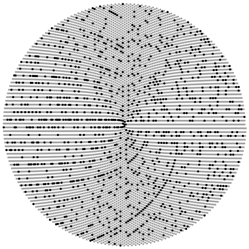
Primes highlighted on a Sacks spiral illustrate their irregular placement among integers; the recent gap estimates require analytic arguments beyond the picture.
Claudio Rocchini / Wikimedia Commons. Unchanged original image. · Image source · CC BY 2.5

On 31 August 2026, Julia Stadlmann submitted a preprint proving that infinitely many consecutive-prime gaps are at most 240. This article examines that particular result and the architecture behind it; it does not identify 240 as the record at the October research cutoff. The numerical change from the earlier 246 bound looks small, but the mathematical point is a way to combine two kinds of distribution information that have different strengths and restrictions. To understand why six units can matter, one has to separate local congruence obstructions, global average estimates and the optimization problem that converts both into a recurring short interval.
A recurring gap is not a bound on all gaps
List the primes in increasing order as p1,p2,p3 and so on. The quantity H1 is the limit inferior of the differences between consecutive primes. A bound H1 at most 240 says that gaps no larger than 240 occur infinitely often. It does not say that every sufficiently large prime has another prime within 240, and it does not assert infinitely many gaps equal to 240. Because only finitely many positive integers lie below that bound, at least one permitted gap value must recur infinitely often, but the theorem need not identify which value.
This distinction is compatible with arbitrarily long gaps. For any positive integer m, the consecutive numbers (m+1)!+2 through (m+1)!+(m+1) are all composite: the term with offset j is divisible by j. Their size is enormous, but their existence already shows that a fixed upper bound cannot govern all prime gaps. A theorem about infinitely many small gaps and a construction of arbitrarily large gaps therefore do not compete. They describe different subsequences. Keeping both examples in mind prevents a limit-inferior statement from becoming a misleading prediction for every prime.
A tuple must survive the obvious obstructions
A standard way to search for clustered primes is to consider shifts n+h1 through n+hk. Some choices cannot all avoid divisibility by a small prime. The shifts {0,1}, for instance, always contain an even member, so they cannot both be prime infinitely often. A tuple is admissible if its shifts omit at least one residue class modulo every prime. This is a necessary local condition for all its translated entries to be prime together. It is not a proof that such simultaneous prime patterns occur.
For a compact hand-checkable example, take shifts {0,2,6}. Modulo two they occupy only residue zero, and modulo three they occupy residues zero and two. For a prime larger than three, three shifts cannot cover every residue class. The tuple is therefore admissible. In contrast, {0,2,4} covers all three residues modulo three, so every translate has a multiple of three. This local arithmetic is cheap to check. The hard part is proving that after surviving every such obstruction, a translated admissible collection contains enough actual primes infinitely often.
Weights turn an existence problem into an inequality
James Maynard's 2013 paper refined the sieve method and proved that arbitrarily many primes can occur in an interval of bounded length, with the interval length depending on the requested number. It also obtained the unconditional recurring-gap bound 600. The key historical role here is the flexible weighting of candidate tuples, which extracts more prime information from distribution estimates than the earlier setup. These statements concern prime clusters and limit inferiors, not a proof of the full prime-tuples conjecture for an individually prescribed admissible tuple.
The basic weighted-average logic can be explained without reproducing the sieve. Assign each candidate n a nonnegative weight w(n), and let C(n) count prime entries in its shifted tuple. If the sum of w(n)C(n) is larger than the sum of w(n), then at least one positively weighted candidate has C(n) greater than one. Otherwise every contribution would satisfy w(n)C(n) at most w(n), contradicting the summed inequality. The analytical work lies in constructing weights whose total mass and prime-weighted mass can both be estimated sharply enough.
Different moduli support different estimates
An arithmetic progression fixes a residue class modulo an integer q. Distribution results compare prime counts in these classes with their expected averages, typically after summing errors across a family of moduli. The word average is essential: it does not promise equally strong control for every individual modulus. A smooth modulus has only relatively small prime factors. Such factorization restrictions can make stronger distribution estimates possible, but they also constrain which terms a sieve construction is allowed to use. A gain in one parameter can therefore bring a loss in another.
Stadlmann's preprint combines the support permitted by the Bombieri–Vinogradov theorem with an additional region using newer estimates for moduli with a substantial smooth factor. The paper develops suitable distribution variants for the mixed terms and reduces the resulting optimization to integrals and a matrix computation. It reports 240 using an admissible 49-tuple, compared with the 50-tuple associated with 246. The statement is unconditional within the preprint. The mechanism is a redesigned combination of usable distribution regions, rather than the observation of an unusually small prime gap in a numerical search.
A finite computation still needs rigorous inputs
The Polymath paper submitted in July 2014 obtained the unconditional bound 246 through generalized Selberg-sieve arguments and extensive calculations. It also separated stronger conclusions that assume versions of the Elliott–Halberstam conjecture from unconditional ones. The unconditional and conjectural regimes therefore answer different logical questions, even when they use closely related sieve weights and appear beside one another in the same abstract. This separation supplies an important reading rule: a small number in a conditional theorem cannot be compared directly with an unconditional bound while dropping the condition. The conjectural distribution statement is part of the theorem's input, not an optional explanatory detail.
A toy optimization illustrates the remaining numerical care. Suppose a proof needs a ratio of two integrals to exceed one. An approximation giving 1.0001 is persuasive only if the certified error is smaller than 0.0001 in the relevant direction. Rounding both numerator and denominator without control can reverse the inequality. Exact arithmetic, interval bounds or analytic error estimates can turn such computations into rigorous steps. Merely running a large floating-point calculation does not. The same distinction separates a proof-assisted optimization from a numerical conjecture about which coefficient choice ought to work.
What this particular improvement teaches
If a translated tuple contains two primes, those primes may not be consecutive within the full prime sequence. Nevertheless, some consecutive pair between them has a gap no larger than the tuple's diameter. This elementary observation bridges a cluster theorem and the recurring consecutive-gap bound. It also explains why optimizing the number of tuple entries and its diameter matters. Removing one required shift can permit a narrower admissible configuration, but only if the analytical inequality still guarantees two surviving primes. Combinatorial and analytic improvements must meet at that interface.
The August result is therefore best understood as evidence that a previously awkward combination of distribution estimates can be made productive. It does not settle the twin-prime conjecture, which asks for infinitely many gaps of two. Nor does it turn sieve weights into an exact description of primality. Further numerical or analytical improvements must certify their own inputs and dependencies. Reading the 240 theorem on its stated date makes its contribution clear: a more efficient use of available progression information can translate into a smaller interval that contains prime pairs infinitely often.
Sources & further reading
Primary papers, project documentation, and research releases used in this article. Publication dates below refer to the sources themselves.
- Bounded gaps between primesarXivPublished Checked
- Small gaps between primesarXivPublished Checked
- Variants of the Selberg sieve, and bounded intervals containing many primesarXivPublished Checked
FOLLOW THE QUESTION
Explore mathematics