MATHEMATICS
Kakeya after the breakthrough: why the 2026 shorter proof matters
A shorter 2026 Kakeya proof clarifies how thin tubes force full fractal dimension in three dimensions, while keeping volume and dimension distinct.
Research checked
Newest cited publication
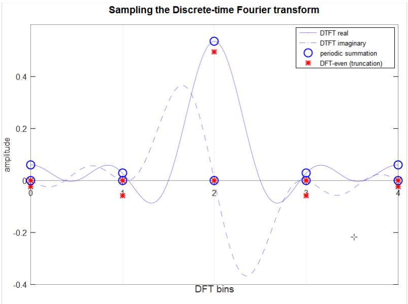
A Fourier-sampling diagram introduces harmonic analysis, one source of tools and questions surrounding Kakeya theory; it does not depict the new geometric proof.
Bob K / Wikimedia Commons. Unchanged original image. · Image source · CC0 1.0

A mathematical breakthrough changes twice: first when a proof establishes a result, and again when its mechanism becomes easier to understand. The three-dimensional Kakeya theorem is undergoing that second change. Hong Wang and Joshua Zahl posted their dimension proof in February 2025. Larry Guth, Wang and Zahl then posted a streamlined argument on January 20, 2026, with a revised version dated October 11. The newer manuscript reorganizes the reduction to an earlier theorem about sticky tube arrangements. Its value is therefore more specific than announcing the same theorem again: it exposes a reusable structure inside a difficult geometric argument.
A needle in every direction
Consider a compact subset of ordinary three-dimensional space that contains a unit line segment pointing in every direction. The segments can be translated separately; they do not have to pass through one common point. The Kakeya dimension theorem says that every such set has both Hausdorff and Minkowski dimension three. The original 2025 paper establishes the result through estimates for unions of thin tubes satisfying a quantitative condition against concentration inside convex sets.
It is useful to construct a deliberately easier comparison. Center every unit segment at the origin and include every orientation. Their union contains a ball of radius one half, so its three-dimensional volume is positive. Allowing separate translations is what makes the actual problem difficult. A proof that only handles the common-center arrangement would leave the essential freedom untouched. Counting available directions alone cannot tell us how ingeniously the translated segments might overlap.
Full dimension leaves room for zero volume
Dimension measures how rapidly covering complexity grows as resolution improves. Volume measures the total amount of space occupied. They answer different questions even when the dimension is an integer. A set can require essentially three-dimensional covering rates while its ordinary volume is zero. Therefore the theorem does not say that every Kakeya set contains a ball, a solid region, or a fixed positive amount of volume.
An elementary sequence explains why this distinction matters. Suppose a hypothetical family of neighborhoods has volume comparable to one divided by the logarithm of one over its thickness. That volume tends to zero, but more slowly than every fixed positive power of thickness. At thickness exp(−100), the logarithmic factor is one hundred; at exp(−1000), it is one thousand. The logarithmic decrease changes constants and slowly varying factors, while a dimension calculation responds to a persistent power. This is an explanatory model, not a construction asserted by the paper.
The accounting problem behind the picture
Replace each line segment by a tube of radius delta and length one. A tube has volume proportional to delta squared. Roughly delta to the power minus two separated directions are needed to sample all directions on the sphere at angular resolution delta. Multiplying those two quantities gives a total tube volume of constant order before overlap is removed. The entire difficulty is how much smaller the union can be than that multiplicity-counted total.
For a finite collection, define the multiplicity at a point as the number of tubes covering it. Integrating multiplicity gives the sum of individual volumes. Integrating the indicator that multiplicity is positive gives the union volume. Their ratio is the average multiplicity on the union. This identity explains why controlling repeated overlap proves a lower bound for occupied space. It also shows why inspecting the maximum overlap at a single point is insufficient: a small exceptional region can have enormous multiplicity without deciding the average.
Following a configuration across scales
Guth's August 2025 outline explains the reduction from the unrestricted problem to the sticky case. Informally, a sticky arrangement has compatible bundles when the tubes are viewed at several resolutions. Nearby directions continue to travel together inside thicker containers instead of reorganizing arbitrarily at every scale. This is a technical geometric property, not an assumption that the segments physically adhere to one another.
Think of viewing a collection of paths first through a coarse pixel grid and then through finer grids. A single coarse image hides whether a bundle later splits neatly or mixes with unrelated bundles. The sequence of images carries additional information. This comparison explains the need for a multiscale argument, although the actual proof uses geometric containers and quantitative estimates rather than image-processing rules. Reducing the general case to sticky behavior is powerful because it channels all possible arrangements into a setting that an earlier theorem can control.
A cleaner dependency structure
The 2026 paper explicitly retains the sticky Kakeya theorem as an input. Its self-contained contribution is the reduction from that theorem to the general volume estimate; it does not replace every earlier ingredient. The authors also state that polynomial partitioning, used in parts of the earlier argument, is no longer needed in this reorganized reduction. Those are meaningful changes in proof architecture rather than a stronger dimension conclusion.
A useful way to read a shorter proof is to draw its dependency graph. Put the desired estimate at the top, intermediate lemmas underneath, and imported theorems at the bottom. Removing one branch can make the structure easier to check even if another substantial theorem remains. Page counts alone conceal this distinction. A ten-page argument importing a hundred-page result is not automatically simpler than a twenty-page argument proving more of its own ingredients. Here the authors identify exactly which reduction they are simplifying, giving readers a more informative comparison.
What an analyst can take from it
The 2025 volume theorem is formulated for tube families with restrictions on how many can fit inside a convex container. That hypothesis is broader than a picture of one segment per direction. It suggests a general strategy: quantify every potential concentration, organize the scales where concentration occurs, and then show that overlap cannot remain excessive throughout the organization. This is an interpretation of the proof's design, not a claim that the same theorem automatically solves every problem involving waves.
Three boundaries should stay visible. The dimension statement concerns three-dimensional Euclidean space. A theorem about sets and their neighborhoods is not, merely by its wording, every possible operator inequality called Kakeya. And replacing straight segments by arbitrary curves changes the geometry. Readers can appreciate the breakthrough without erasing those boundaries. The most productive next use of the shorter argument is to understand which pieces depend specifically on straightness, convexity and three dimensions, and which pieces are general methods for handling concentration. That is how a solved problem becomes a source of further mathematics.
Reading the exponent without overstating it
There is a useful calculation behind the phrase full dimension. Suppose a neighborhood of thickness delta can be covered by N cubes of side delta. Its volume is at most a constant times N times delta cubed. A lower bound of order delta to the power beta therefore forces N to be at least of order delta to the power minus three plus beta. If such bounds are available for every positive beta, no fixed smaller exponent can describe the covering growth. This is the basic exponent bookkeeping behind a Minkowski-dimension conclusion; establishing Hausdorff dimension requires the additional covering control supplied by the theorem.
For example, a hypothetical bound valid only with beta equal to one tenth would point toward a covering exponent of 2.9, not automatically three. Being able to make beta arbitrarily small changes the conclusion. At the same time, the constant may depend on beta, so one cannot set beta equal to zero inside the estimate and conclude a uniform positive volume. The order of these operations matters: first fix a positive loss, then pass to sufficiently fine scales, and only afterward infer the limiting dimension.
Sources & further reading
Primary papers, project documentation, and research releases used in this article. Publication dates below refer to the sources themselves.
- A streamlined proof of the Kakeya set conjecture in ℝ³arXivPublished Checked
- Volume estimates for unions of convex sets, and the Kakeya set conjecture in three dimensionsarXivPublished Checked
- Outline of the Wang-Zahl proof of the Kakeya conjecture in ℝ³arXivPublished Checked
FOLLOW THE QUESTION
Explore mathematics