MATHEMATICS
From colliding spheres to fluid equations: what Hilbert’s sixth problem now means
A close look at the 2025 hard-sphere derivation of fluid equations, the long-time collision argument behind it, and the precise limits of the result.
Research checked
Newest cited publication
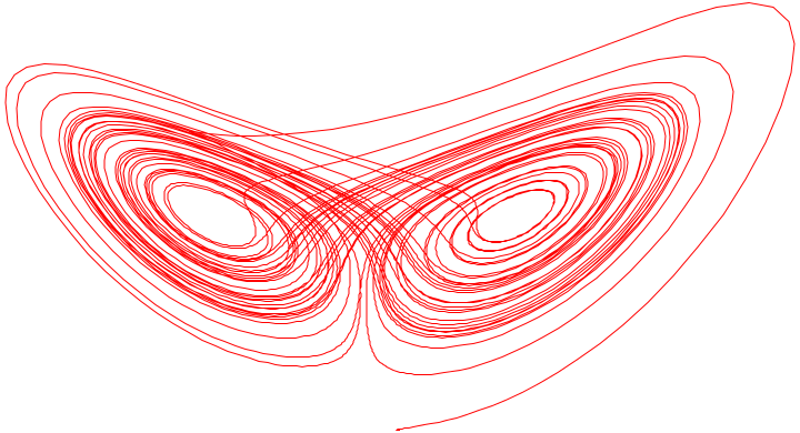
A Lorenz-system trajectory provides background imagery for nonlinear evolution; the hard-sphere dynamics and rigorous fluid limits discussed here are different mathematical models.
Cepheus / Wikimedia Commons. Unchanged original image. · Image source · Public domain (released by the creator)

A gas can be described by tracking every molecule, by following a distribution of velocities, or by measuring fields such as density and temperature. These descriptions do not simply become equivalent because all three are useful. Proving their relationship is a mathematical problem. A March 2025 preprint by Yu Deng, Zaher Hani and Xiao Ma supplied a major link for a dilute hard-sphere gas, with a revised long-time companion paper following in July. An author’s Oxford colloquium in May 2026 continued to present the work as a central development in Hilbert’s program. Understanding the achievement requires keeping the model, the limits and the time interval in view.
Three descriptions with different unknowns
At the particle level, a state lists positions and velocities. Between collisions, hard spheres move freely; an elastic collision changes velocities while conserving total momentum and kinetic energy. At the kinetic level, the unknown is a density f depending on time, position and velocity. Integrating f over velocities gives the local particle density. Multiplying by velocity before integrating gives momentum density. The fluid level retains only a small collection of such moments. This is a substantial reduction of information, so a derivation must explain why information discarded at each step does not return in a way that changes the answer.
Consider two equally populated velocity groups moving at equal speeds in opposite directions. Their average velocity is zero, but their kinetic energy is positive. A fluid description that recorded only the mean velocity would confuse this gas with one whose particles were all stationary. Temperature and stress record some of the missing information. This elementary example explains why passing from a velocity distribution to fluid fields involves a closure problem: the evolution of a low moment generally depends on higher moments. A useful limit must justify a particular closure rather than assume that averaging automatically produces a closed equation.
The two limiting operations do different jobs
The March 3, 2025 preprint derives compressible Euler and incompressible Navier–Stokes–Fourier descriptions through Boltzmann kinetic theory. Its particle model is hard spheres undergoing elastic collisions, and the kinetic argument is extended to two- and three-dimensional periodic domains. For the incompressible Navier–Stokes–Fourier derivation, the initial particle distribution is close to global equilibrium. The theorem uses an iterated limit: first the Boltzmann–Grad limit with collision rate fixed, then a separate hydrodynamic limit as that rate grows. These results are not an assertion that every liquid, interacting plasma or microscopic material has been reduced to the same theorem. The authors’ title refers to the fluid-mechanics component of Hilbert’s sixth problem; the broader historical request for an axiomatization of physics is larger.
The distinction between the limits can be seen by dimensional counting. If N spheres have diameter ε in dimension d, a collision cross-section scales like ε raised to d minus one. Keeping N times that quantity controlled can preserve an appreciable collision rate. The occupied volume instead scales like N times ε raised to d, which then has an additional factor ε and tends to zero. A gas may therefore have frequent collisions while still occupying a vanishing volume fraction. Passing afterward to a macroscopic scale is a second operation. Exchanging these limits without an estimate would be an additional theorem, not an innocent change of notation.
Why the time interval was the difficult bridge
The companion work, initially submitted in August 2024 and substantially revised on July 18, 2025, extends the microscopic derivation of Boltzmann’s equation beyond the short interval of Lanford’s classical theorem. The important qualification is the strong kinetic lifespan: the corresponding strong Boltzmann solution must exist on the time interval under consideration, within the theorem’s regularity and velocity-tail assumptions. “Arbitrarily long” here does not mean that the authors prove every Boltzmann solution remains smooth forever. It means the derivation can follow that strong kinetic solution for any fixed admissible interval instead of stopping at a universal short-time barrier.
A bookkeeping analogy helps explain that barrier. After one collision, a particle’s velocity depends on a partner. Following the partner backward introduces its earlier partners, and the dependency tree expands. If two branches meet again, a recollision creates a correlation that independent-particle bookkeeping misses. Counting each possible history separately becomes ineffective over long times, even when each individual exceptional event looks unlikely. The proof must estimate whole families of correlated histories together. An exponential number of small terms can have a large sum; a long-time theorem needs a mechanism that controls their collective contribution.
A proof that remembers enough of the past
The revised companion paper describes its organizing device as a long-time cumulant ansatz, with partial time expansions and diagrammatic objects called molecules. Cumulants measure the part of a joint distribution that cannot be reconstructed from lower-order independent pieces. The authors keep the collision history needed to control these quantities and prove their smallness through a combinatorial cutting argument. The lesson is not that molecular correlations disappear exactly. Rather, their contribution is quantitatively controlled in the limiting observables that the theorem studies.
For a simple probability calculation, independent binary variables X and Y satisfy an average of their product equal to the product of their averages. Their difference is a covariance, the simplest connected correction. Adding a third variable produces higher connected corrections that cannot be summarized by three separate means. A kinetic proof has to handle analogous corrections for many interacting trajectories, with geometry and time ordering attached. This explanation is only an analogy, not the authors’ full construction, but it shows why estimating a one-particle distribution alone cannot establish microscopic independence over the required interval.
Derivation is different from solving a fluid equation
The Oxford lecture abstract, scheduled for May 8, 2026, emphasizes the route from Newtonian particles to kinetic and then fluid equations, and the connection to earlier work on wave turbulence. That provides a useful map of the research program. A derivation theorem answers whether one description approximates another under specified assumptions. An existence or regularity theorem answers whether the target equation has a solution with specified properties. These questions interact, but one cannot substitute for the other. In particular, deriving a Navier–Stokes–Fourier regime does not by itself settle unrestricted three-dimensional Navier–Stokes regularity.
An error estimate illustrates the logical separation. Suppose a particle observable differs from a smooth continuum field by at most a constant times a small parameter on a fixed interval. If the continuum field ceases to satisfy the assumptions at a later time, the estimate no longer supplies information there. Increasing the number of particles does not repair a missing hypothesis about the continuum solution. Conversely, a beautiful continuum existence theorem says nothing about whether a chosen molecular model converges to it. Both sides of the bridge need their own mathematical support.
How to evaluate the next claim in this area
A short April 2025 comment by Shan Gao challenges broad physical interpretations of the hard-sphere result, focusing on dilution and correlations. It should be read as a separate author’s critique of scope, not as an established refutation of the derivation. The clean way to evaluate such discussion is to separate three propositions: the theorem’s hypotheses, the proof that its conclusion follows, and the claim that its model captures a particular physical material. A limitation of the third proposition does not automatically invalidate the first two.
Future extensions can be judged concretely: change the interaction law, include a boundary, weaken the data assumptions, improve quantitative rates, or justify a different order of limits. Each change may expose correlations absent from the current setting. For a reader, the most productive question is therefore which approximation is controlled and on what interval. The current work makes an unusually long microscopic-to-macroscopic argument possible for a precise gas model. Its power becomes clearer, rather than smaller, when that precision is kept visible.
Sources & further reading
Primary papers, project documentation, and research releases used in this article. Publication dates below refer to the sources themselves.
- Hilbert's sixth problem: derivation of fluid equations via Boltzmann's kinetic theoryarXivPublished Checked
- Long time derivation of the Boltzmann equation from hard sphere dynamicsarXivPublished Checked
- On Hilbert’s sixth problem: from particles to wavesUniversity of Oxford Mathematical InstitutePublished Checked
- Comment on "Hilbert's Sixth Problem: Derivation of Fluid Equations via Boltzmann's Kinetic Theory" by Deng, Hani, and MaarXivPublished Checked
FOLLOW THE QUESTION
Explore mathematics