PHYSICS
The 1965 Microwave Background Discovery: How an Unwanted Signal Became Cosmology
Follow the 1965 microwave discovery from calibrated antenna noise to a hot-universe interpretation, and see why measuring a spectrum required further experiments.
Research checked
Newest cited publication
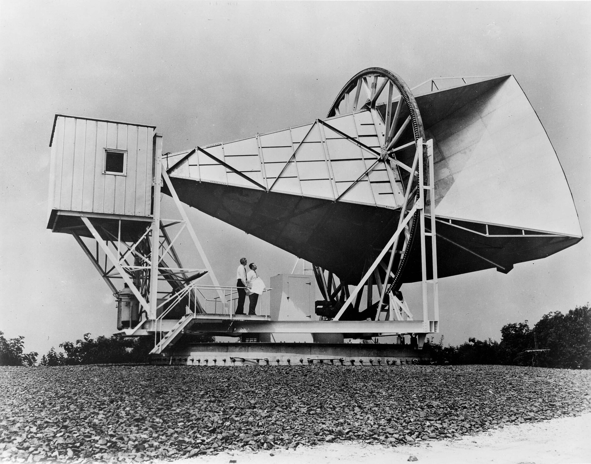
An archival photograph shows the Holmdel horn antenna used by Penzias and Wilson. Their investigation of its persistent microwave signal helped establish the cosmic microwave background in 1965.
NASA · Image source · NASA educational and editorial media reuse permission

The discovery of the cosmic microwave background was not a photograph of the beginning of the universe. It was a carefully investigated surplus of radio noise. In July 1965, Arno Penzias and Robert Wilson reported an unexplained antenna temperature at Bell Laboratories, while a companion paper by Robert Dicke, James Peebles, Peter Roll, and David Wilkinson discussed a possible cosmological interpretation. The observations included measurements made during 1964 and 1965. This distinction between observing an anomaly and explaining it is central to the achievement. A signal that initially frustrated an instrument measurement became evidence about the universe because researchers made its terrestrial alternatives increasingly difficult to sustain.
An unexplained contribution, rather than a complete cosmic model
Penzias and Wilson worked with a horn-reflector antenna at Crawford Hill in New Jersey. Their report concerned observations at 4,080 megacycles per second, now written as 4.08 gigahertz. After accounting for known contributions, they found an excess equivalent to 3.5 kelvin, with an estimated uncertainty of 1 kelvin. The reported excess was approximately direction-independent and unpolarized within their observational limits. Those qualifications matter: the experiment did not establish perfect uniformity across every direction or every frequency.
The important object was the unexplained remainder after an accounting exercise. A receiver can respond to radiation from the sky, the atmosphere, the ground, and its own physical components. All those contributions can arrive as fluctuating electrical power. Finding an excess therefore requires more than noticing that the receiver makes noise. It requires establishing the expected contributions well enough that their plausible errors cannot comfortably absorb the remainder. The measurement's intellectual difficulty was partly the difficulty of knowing the apparatus.
A temperature scale can describe a signal without touching it
An antenna temperature is a way of expressing received noise power using a thermal reference. It does not mean that someone inserted a thermometer into a distant cloud. Wilson's later Nobel lecture explains the calibration idea through an equivalent warm electrical source. Two sources that supply the same noise power can be assigned the same equivalent temperature even if their microscopic origins differ. Calling a residual a temperature therefore describes its measured strength; it does not, by itself, establish a thermal cosmic origin.
For example, in the usual low-frequency thermal-noise approximation, one matched mode supplies power equal to Boltzmann's constant multiplied by temperature and bandwidth. A 3-kelvin source observed over an illustrative bandwidth of one megahertz gives approximately 4.14 times ten to the minus seventeen watts. That is an extraordinarily small power to distinguish from instrument contributions. These numbers describe a simplified calibration calculation, not the actual bandwidth or detailed sensitivity of the discovery receiver. The example shows why a cold reference and low-loss components matter.
The uncertainty belongs to the whole noise budget
The 1965 letter gives a zenith antenna temperature of 6.7 kelvin, an atmospheric contribution of 2.3 kelvin, and a calculated contribution of 0.9 kelvin from antenna losses and unwanted response. Subtracting gives the reported 3.5-kelvin remainder. The atmospheric term was investigated by changing elevation, which changes the path through the atmosphere. This is a physical diagnostic: an atmospheric explanation should respond to that controlled change in a predictable way.
Consider a separate calibration example. Suppose a total reading is 10 units and an estimated background is 7 units, each with independent uncertainty of 0.5 units. Their difference is 3 units, but its uncertainty is about 0.71 units, found by adding the two variances and taking the square root. Repeating only the total reading cannot remove the background uncertainty. If the errors share a calibration offset, independence also fails. A small residual is convincing when the entire subtraction, including dependencies between terms, has been tested.
Changing the experiment helps distinguish possible origins
A useful astronomical source often reveals itself by changing as an antenna scans. A nearly uniform background creates the opposite problem: it can resemble an unchanging instrumental offset. Wilson's firsthand account describes the extensive attention paid to the antenna's response and unwanted radiation. A steady contribution is not automatically cosmic merely because familiar bright objects cannot explain it. The stability that makes a cosmological background plausible also makes a stable calibration problem particularly important to exclude.
Imagine measuring a room's light level with a detector that has an unknown electrical offset. Pointing it toward several equally bright walls will not separate the offset from genuine illumination. Covering the detector, changing a reference source, or altering its sensitivity introduces a new comparison. Radio astronomy uses more sophisticated versions of this logic. The strongest test changes a suspected contaminant while preserving the desired signal, or changes the desired signal in a way that an instrumental offset cannot imitate. Repetition without such a distinction can deliver precision without resolving origin.
Expansion changes a thermal spectrum in a specific way
Dicke, Peebles, Roll, and Wilkinson's companion paper discussed radiation surviving from a much hotter cosmic state. It explicitly noted that additional measurements were needed to determine the spectrum. Its physical proposal was stronger than saying that the sky should contain some extra radio emission: expansion could cool radiation while preserving a thermal, or blackbody, form. That supplied a pattern against which further observations could be compared. The same article explored cosmological possibilities that should not all be mistaken for today's accepted model.
The cooling argument is simple to visualize. If cosmic expansion doubles every wavelength, each photon's energy halves. A fixed population of photons also occupies eight times as much physical volume when every spatial dimension doubles. Its energy density therefore falls by a factor of sixteen. A blackbody's energy density depends on the fourth power of its temperature, so a halved temperature gives exactly that factor. The agreement connects expansion, photon energy, and thermal radiation; it is more informative than assigning a temperature to one isolated frequency.
The later blackbody test answered a different question
Many distinct radiation mechanisms can produce the same intensity at one frequency. Distinguishing them requires a spectral shape. The Cosmic Background Explorer satellite supplied an especially clear later test: a paper published on May 10, 1990 reported a spectrum from its Far Infrared Absolute Spectrophotometer, or FIRAS. The preliminary measurement fitted a blackbody at 2.735 kelvin, with uncertainty of 0.06 kelvin, and constrained deviations to less than one percent of the peak intensity over its stated spectral range.
The instrument compared sky radiation with a reference blackbody and operated outside Earth's atmosphere. That comparison addressed difficulties different from merely repeating the original radio measurement. Think of identifying a musical instrument: one loudness reading cannot tell a violin from a flute, but the distribution of power across frequencies adds discriminating structure. Similarly, the background's thermal spectrum established an important property of the signal without turning the 1965 apparatus into an instrument that had already measured that spectrum. Discovery and characterization remained separate experimental achievements.
A durable result can outlive its first interpretations
The paired 1965 papers distribute the scientific work clearly. Penzias and Wilson reported the unexpected measurement; the Princeton group supplied a developed hot-universe interpretation and plans for further spectral observations. Wilson's 1978 lecture offers a later participant's account, rather than a replacement for the contemporary measurement record. Reading those records together avoids reducing the discovery to either a fortunate accident or a theory triumph. Preparation made the anomaly visible, calibration made it credible, and physical interpretation made it cosmologically useful.
The result did not by itself determine the universe's age, all its ingredients, or the origin of its initial conditions. Its lasting force came from creating additional tests: a thermal spectrum, consistency across instruments, and increasingly detailed checks of directional structure. That is a practical lesson for evaluating discoveries elsewhere in physics. A persuasive anomaly does not end with a remainder that lacks an explanation. It motivates a physical account whose consequences can be measured through different experimental arrangements.
Sources & further reading
Primary papers, project documentation, and research releases used in this article. Publication dates below refer to the sources themselves.
- A Measurement of Excess Antenna Temperature at 4080 Mc/s.A. A. Penzias and R. W. Wilson / The Astrophysical Journal; NASA ADS archivePublished Checked
- Cosmic Black-Body Radiation.R. H. Dicke, P. J. E. Peebles, P. G. Roll, and D. T. Wilkinson / The Astrophysical Journal; NASA ADS archivePublished Checked
- The Cosmic Microwave Background RadiationRobert W. Wilson / Nobel FoundationPublished Checked
- A preliminary measurement of the cosmic microwave background spectrum by the Cosmic Background Explorer (COBE) satelliteJ. C. Mather and collaborators / The Astrophysical Journal; NASA ADS archivePublished Checked
FOLLOW THE QUESTION
Explore physics